文章目录

0. 实验环境
本实验使用了PyTorch深度学习框架,相关操作如下:
conda create -n DL python==3.11
conda activate DL
conda install pytorch torchvision torchaudio pytorch-cuda=12.1 -c pytorch -c nvidia
conda install matplotlib
conda install pillow numpy
| 软件包 | 本实验版本 |
|---|---|
| matplotlib | 3.8.0 |
| numpy | 1.26.3 |
| pillow | 10.0.1 |
| python | 3.11.0 |
| torch | 2.1.2 |
| torchaudio | 2.1.2 |
| torchvision | 0.16.2 |
1. 理论基础
二维卷积运算是信号处理和图像处理中常用的一种运算方式,当给定两个二维离散信号或图像
f
(
x
,
y
)
f(x, y)
f(x,y) 和
g
(
x
,
y
)
g(x, y)
g(x,y),其中
f
(
x
,
y
)
f(x, y)
f(x,y) 表示输入信号或图像,
g
(
x
,
y
)
g(x, y)
g(x,y) 表示卷积核。二维卷积运算可以表示为:
h
(
x
,
y
)
=
∑
m
∑
n
f
(
m
,
n
)
⋅
g
(
x
−
m
,
y
−
n
)
h(x, y) = \sum_{m}\sum_{n} f(m, n) \cdot g(x-m, y-n)
h(x,y)=m∑n∑f(m,n)⋅g(x−m,y−n)其中
∑
m
∑
n
\sum_{m}\sum_{n}
∑m∑n 表示对所有
m
,
n
m, n
m,n 的求和,
h
(
x
,
y
)
h(x, y)
h(x,y) 表示卷积后的输出信号或图像。
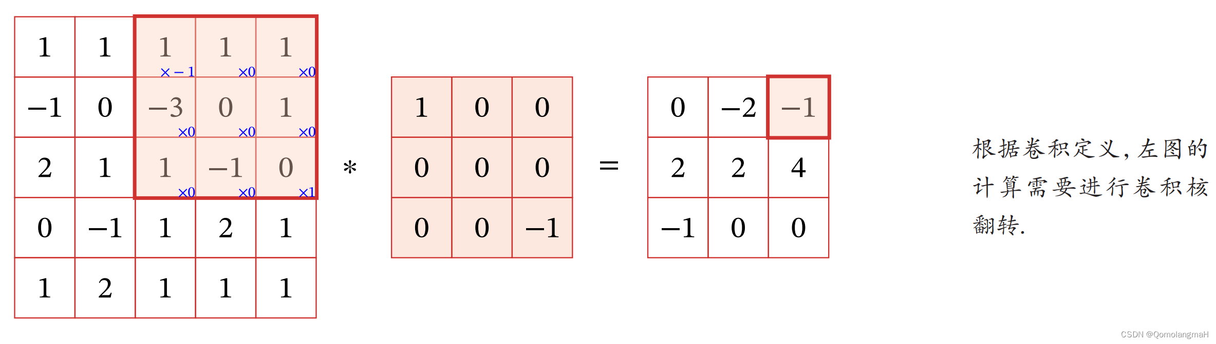
在数学上,二维卷积运算可以理解为将输入信号或图像
f
(
x
,
y
)
f(x, y)
f(x,y) 和卷积核
g
(
x
,
y
)
g(x, y)
g(x,y) 进行对应位置的乘法,然后将所有乘积值相加得到输出信号或图像
h
(
x
,
y
)
h(x, y)
h(x,y)。这个过程可以用于实现一些信号处理和图像处理的操作,例如模糊、边缘检测、图像增强等。
详见:【深度学习】Pytorch 系列教程(七):PyTorch数据结构:2、张量的数学运算(5):二维卷积及其数学原理
1.1 滤波器(卷积核)
在图像处理中,卷积经常作为特征提取的有效方法.一幅图像在经过卷积操作后得到结果称为特征映射(Feature Map)。图5.3给出在图像处理中几种常用的滤波器,以及其对应的特征映射.图中最上面的滤波器是常用的高斯滤波器,可以用来对图像进行平滑去噪;中间和最下面的滤波器可以用来提取边缘特征。
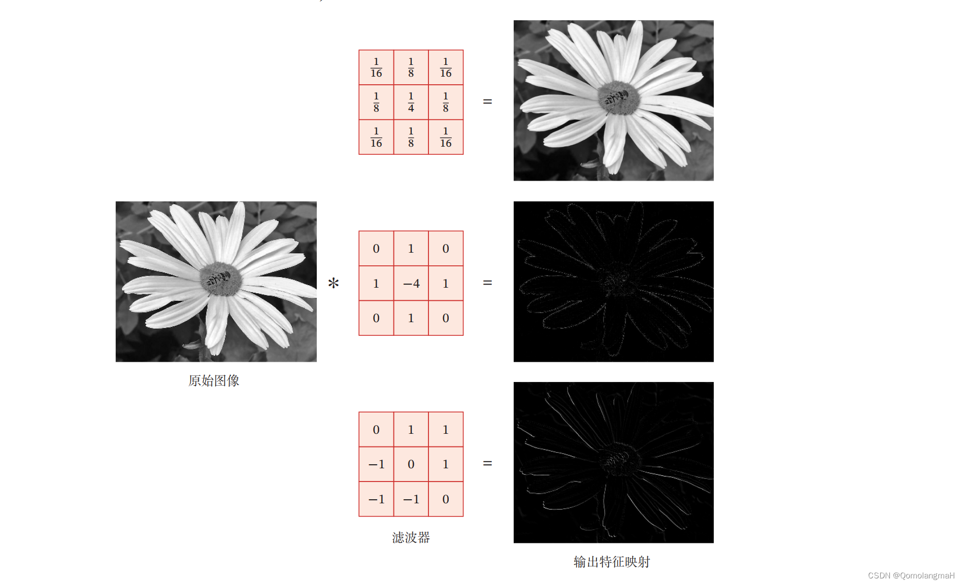
# 高斯滤波~平滑去噪
conv_kernel1 = torch.tensor([[1/16, 1/8, 1/16],
                            [1/8, 1/4, 1/8],
                            [1/16, 1/8, 1/16]], dtype=torch.float).unsqueeze(0).unsqueeze(0)
# 提取边缘特征
conv_kernel2 = torch.tensor([[0, 1, 0],
                            [1, -4, 1],
                            [0, 1, 0]], dtype=torch.float).unsqueeze(0).unsqueeze(0)
conv_kernel3 = torch.tensor([[0, 1, 1],
                            [-1, 0, 1],
                            [-1, -1, 0]], dtype=torch.float).unsqueeze(0).unsqueeze(0)
print(conv_kernel1.size())
- 上述均为3x3的单通道卷积核,需要拓展为四维张量(PyTorch就是这么设计的~)
1.2 PyTorch:卷积操作
def conv2d(img_tensor, conv_kernel):
    convolved_channels = []
    for i in range(3):
        channel_input = img_tensor[:, i, :, :]  # 取出每个通道的输入
        convolved = F.conv2d(channel_input, conv_kernel, padding=1)
        convolved_channels.append(convolved)

    # 合并各通道卷积后的结果
    output = torch.cat(convolved_channels, dim=1)
    # 将张量转换为NumPy数组,进而转换为图像
    output_img = output.squeeze().permute(1, 2, 0).numpy().astype(np.uint8)
    output_img = Image.fromarray(output_img)
    return output_img
2. 图像处理
2.1 图像读取
img = Image.open('1.jpg')
# img = img.resize((128, 128))  # 调整图像大小

img_tensor = torch.tensor(np.array(img), dtype=torch.float).permute(2, 0, 1).unsqueeze(0)

print(img_tensor.shape)
- 将图像转换为PyTorch张量:将通道顺序从HWC转换为CHW,并在第一个维度上增加一个维度~卷积操作使用四维张量
2.2 查看通道
本部分内容纯属没事儿闲的~
img = Image.open('1.jpg')
img_tensor = torch.tensor(np.array(img), dtype=torch.float).permute(2, 0, 1).unsqueeze(0)
channel1 = img_tensor[:, 0, :, :]  # 提取每个通道
channel2 = img_tensor[:, 1, :, :]
channel3 = img_tensor[:, 2, :, :]
plt.figure(figsize=(12, 12))
plt.subplot(1, 4, 1)
plt.imshow(img)
plt.axis('off')
plt.subplot(1, 4, 2)
channel1_img = channel1.squeeze().numpy().astype(np.uint8)
channel1_img = Image.fromarray(channel1_img)
plt.imshow(channel1_img)
plt.axis('off')
plt.subplot(1, 4, 3)
channel2_img = channel2.squeeze().numpy().astype(np.uint8)
channel2_img = Image.fromarray(channel2_img)
plt.imshow(channel2_img)
plt.axis('off')
plt.subplot(1, 4, 4)
channel3_img = channel3.squeeze().numpy().astype(np.uint8)
channel3_img = Image.fromarray(channel3_img)
plt.imshow(channel3_img)
plt.axis('off')


2.3 图像处理
def plot_img(img_tensor):
    output_img1 = conv2d(img_tensor, conv_kernel1)
    output_img2 = conv2d(img_tensor, conv_kernel2)
    output_img3 = conv2d(img_tensor, conv_kernel3)

    plt.subplot(2, 2, 1)
    plt.title('原始图像', fontproperties=font)
    plt.imshow(img)
    plt.axis('off')
    plt.subplot(2, 2, 2)
    plt.title('平滑去噪', fontproperties=font)
    plt.imshow(output_img1)
    plt.axis('off')
    plt.subplot(2, 2, 3)
    plt.imshow(output_img2)
    plt.title('边缘特征1', fontproperties=font)
    plt.axis('off')
    plt.subplot(2, 2, 4)
    plt.imshow(output_img3)
    plt.title('边缘特征2', fontproperties=font)
    plt.axis('off')
    plt.show()
font = FontProperties(fname='C:\Windows\Fonts\simkai.ttf', size=16)  # 使用楷体
plt.figure(figsize=(12, 12))  # 设置图大小12*12英寸
plot_img(img_tensor)


- 如图所示,图像提取边缘特征效果明显
- 但图片过于高清,plt输出的(12英寸)原始图像、平滑去噪图像都很模糊~,下面会先降低像素,然后进行去模糊去噪实验
- 原图为

3. 图像去模糊
img = Image.open('2.jpg')
img = img.resize((480, 480))  # 调小图像~先使原图变模糊
img_tensor = torch.tensor(np.array(img), dtype=torch.float).permute(2, 0, 1).unsqueeze(0)
conv_kernel4 = torch.tensor([[0, 0, 0],
                            [0, 2, 0],
                            [0, 0, 0]], dtype=torch.float).unsqueeze(0).unsqueeze(0)
conv_kernel5 = torch.ones(3, 3).unsqueeze(0).unsqueeze(0)/9
# print(conv_kernel4-conv_kernel5)
font = FontProperties(fname='C:\Windows\Fonts\simkai.ttf', size=32)
plt.figure(figsize=(32, 32))
plt.subplot(2, 2, 1)
plt.title('原始图像', fontproperties=font)
plt.imshow(img)
plt.axis('off')
plt.subplot(2, 2, 2)
plt.title('线性滤波-2', fontproperties=font)
plt.imshow(conv2d(img_tensor, conv_kernel4))
plt.axis('off')
plt.subplot(2, 2, 3)
plt.imshow(conv2d(img_tensor, conv_kernel5))
plt.title('均值滤波器:模糊', fontproperties=font)
plt.axis('off')
plt.subplot(2, 2, 4)
plt.imshow(conv2d(img_tensor, conv_kernel4-conv_kernel5))
plt.title('锐化滤波器:强调局部差异', fontproperties=font)
plt.axis('off')
plt.show()

4. 图像去噪
4.1 添加随机噪点
img = Image.open('1.jpg')
img = img.resize((640, 640))  # 调小图像~先使原图变模糊
img_tensor = torch.tensor(np.array(img), dtype=torch.float).permute(2, 0, 1).unsqueeze(0)


noise = torch.randn_like(img_tensor)    # 与图像相同大小的随机标准正态分布噪点
noisy_img_tensor = img_tensor + noise   # 将噪点叠加到图像上
noisy_img = noisy_img_tensor.squeeze(0).permute(1, 2, 0).to(dtype=torch.uint8)
noisy_img = Image.fromarray(noisy_img.numpy())
4.2 图像去噪
# conv_kernel1 = torch.tensor([[1/16, 1/8, 1/16],
#                             [1/8, 1/4, 1/8],
#                             [1/16, 1/8, 1/16]], dtype=torch.float).unsqueeze(0).unsqueeze(0)
# # 生成随机3x3高斯分布
# random_gaussian = torch.randn(3, 3).unsqueeze(0).unsqueeze(0)
# print(random_gaussian)
font = FontProperties(fname='C:\Windows\Fonts\simkai.ttf', size=32)  # 使用楷体
plt.figure(figsize=(32, 32))
plt.subplot(1, 3, 1)
plt.title('原始图像', fontproperties=font)
plt.imshow(img)
plt.axis('off')
plt.subplot(1, 3, 2)
plt.title('噪点图像', fontproperties=font)
plt.imshow(noisy_img)
plt.axis('off')
plt.subplot(1, 3, 3)
plt.title('去噪图像', fontproperties=font)
plt.imshow(conv2d(noisy_img_tensor, conv_kernel1))
plt.axis('off')
plt.show()


