@TOC

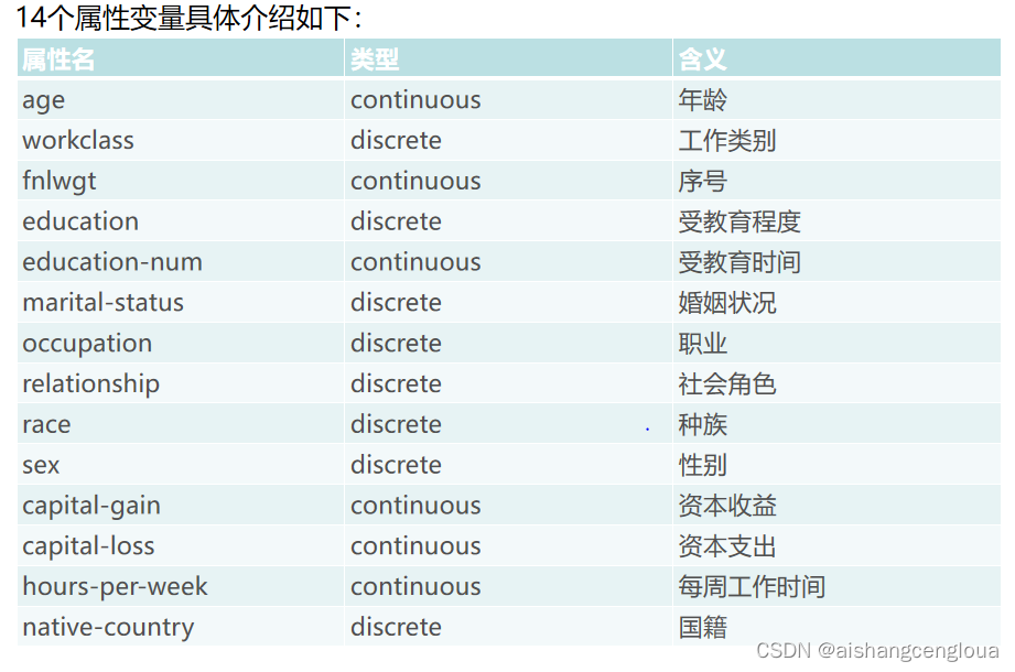
一、数据集

数据集介绍

Adult数据集是一个经典的数据挖掘项目的的数据集，该数据从美国1994年人口普查数据库中抽取而来，因此也称作“人口普查收入”数据集，共包含48842条记录，年收入大于 50k$ 的占比23.93%年收入小于 50k$ 的占比76.07%，数据集已经划分为训练数据32561条和测试数据16281条。该数据集类变量为年收入是否超过 50k$ ，属性变量包括年龄、工种、学历、职业等14类重要信息，其中有8类属于类别离散型变量，另外6类属于数值连续型变量。该数据集是一个分类数据集，用来预测年收入是否超过50k$。下载地址点这里

数据集预处理及分析

因为是csv数据，所以主要采用pandas和numpy库来进行预处理，首先数据读取以及查看是否有缺失值

import pandas as pd 
import numpy as np

df = pd.read_csv('adult.csv', header = None, names = ['age', 'workclass', 'fnlwgt', 'education', 'education-num', 'marital-status', 'occupation', 'relationship',  'race', 'sex', 'capital-gain', 'capital-loss', 'hours-per-week', 'native-country', 'income'])
df.head()
df.info()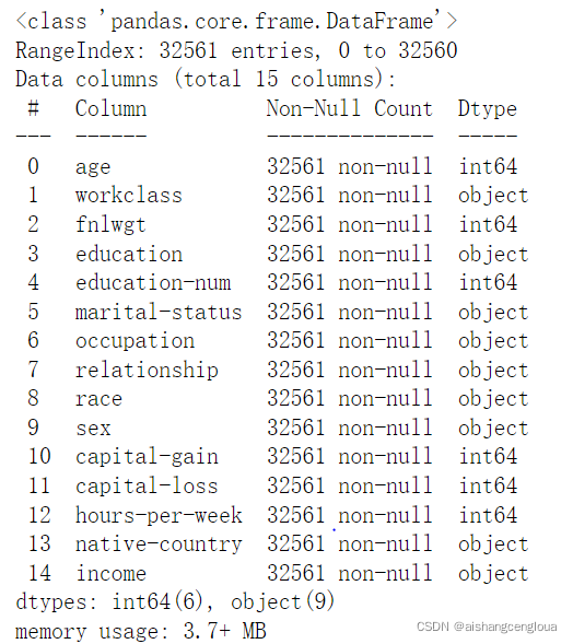

虽然上面查看数据是没有缺失值的，但其实是因为缺失值的是" ?"，而info()检测的是NaT或者Nan的缺失值。注意问号前面还有空格。

df.apply(lambda x : np.sum(x == " ?"))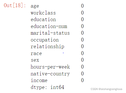

分别是居民的工作类型workclass（离散型）缺1836、职业occupation（离散型）缺1843和国籍native-country（离散型）缺583。离散值一般填充众数，但是在此之前要先将缺失值转化成nan或者NaT。同时因为收入可以分为两种类型，则将>50K的替换成1，<=50K的替换成0

df.replace(" ?", pd.NaT, inplace = True)
df.replace(" >50K", 1, inplace = True)
df.replace(" <=50K", 0, inplace = True)
trans = {'workclass' : df['workclass'].mode()[0], 'occupation' : df['occupation'].mode()[0], 'native-country' : df['native-country'].mode()[0]}
df.fillna(trans, inplace = True)
df.describe()

<center>

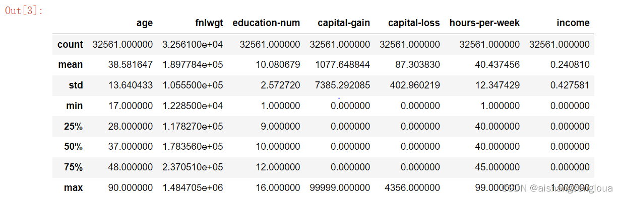
由上表可知，75%以上的人是没有资本收益和资本输出的，所以这两列是属于无关属性的，此外还包括序号列，应删除这三列。所以我们只需关注这三列之外的数据即可。

df.drop('fnlwgt', axis = 1, inplace = True)
df.drop('capital-gain', axis = 1, inplace = True)
df.drop('capital-loss', axis = 1, inplace = True)
df.head()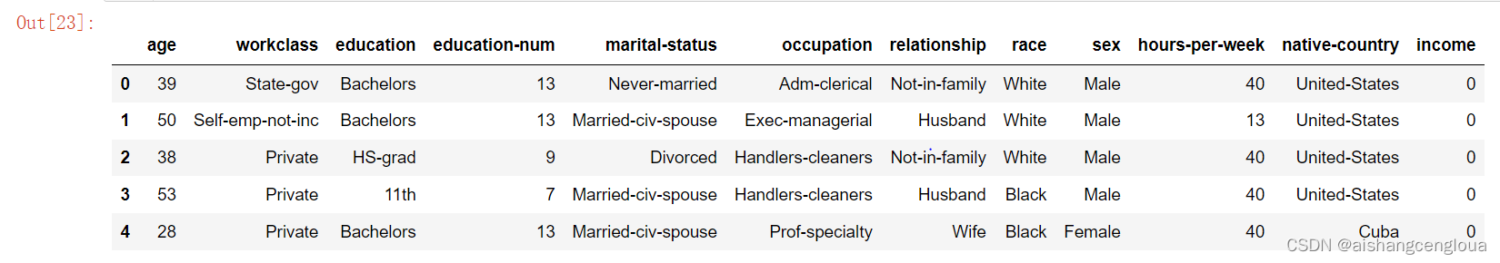

import matplotlib.pyplot as plt

plt.scatter(df["income"], df["age"])
plt.grid(b = True, which = "major", axis = 'y')
plt.title("Income distribution by age (1 is >50K)")
plt.show()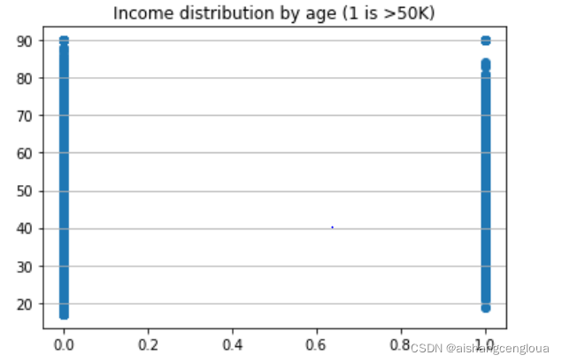

能看出对于中高年龄的人来说收入>50K是比<=50K的少

df["workclass"].value_counts()

income_0 = df["workclass"][df["income"] == 0].value_counts()
income_1 = df["workclass"][df["income"] == 1].value_counts()
df1 = pd.DataFrame({" >50K" : income_1, " <=50K" : income_0})
df1.plot(kind = 'bar', stacked = True)
plt.title("income distribution by Workclass")
plt.xlabel("workclass")
plt.ylabel("number of person")
plt.show()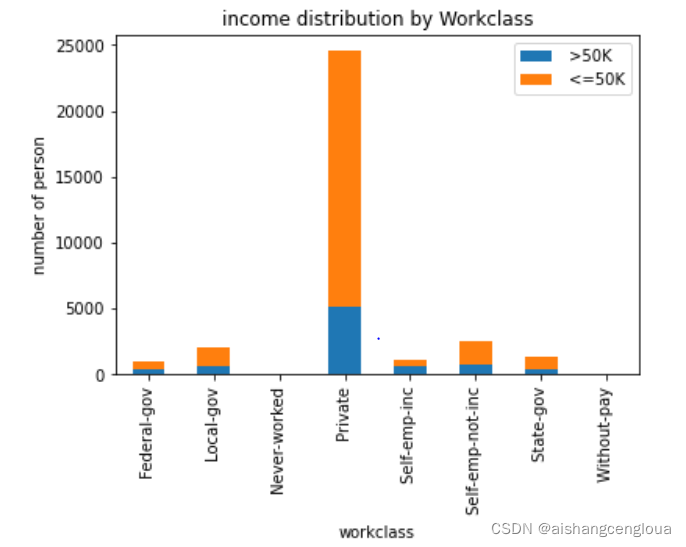

观察工作类型对年收入的影响。工作类别为Private的人在两种年收入中都是最多的，但是>50K和<=50K的比例最高的是Self-emp-inc

df1 = df["hours-per-week"].groupby(df["workclass"]).agg(['mean','max','min'])
df1.sort_values(by = 'mean', ascending = False)
df1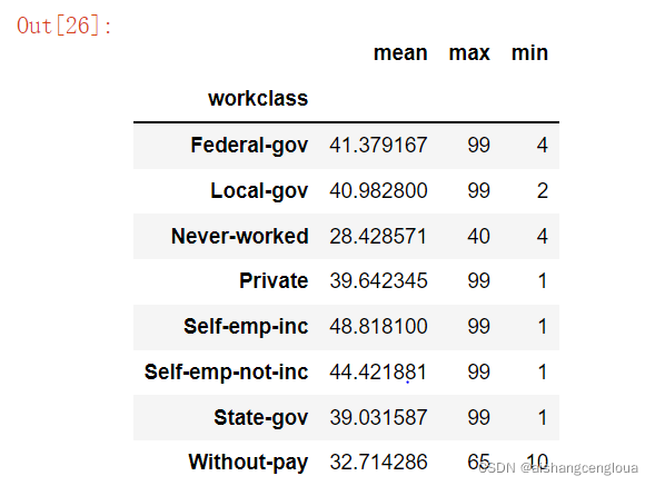

用工作类别对每周工作时间进行分组，计算每组的均值，最大、小值，并且按均值进行排序。能看出工作类别是Federal-gov的人平均工作时间最长，但其的高收入占比并不是最高的。

income_0 = df["education"][df["income"] == 0].value_counts()
income_1 = df["education"][df["income"] == 1].value_counts()
df1 = pd.DataFrame({" >50K" : income_1, " <=50K" : income_0})
df1.plot(kind = 'bar', stacked = True)
plt.title("income distribution by Workclass")
plt.xlabel("education")
plt.ylabel("number of person")
plt.show()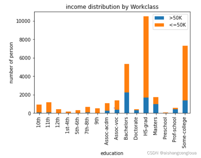

统计受教育程度对年收入的影响，对于程度是Bachelors来说，两种收入的人数是比较接近的，收入比也是最大的

income_0 = df["education-num"][df["income"] == 0]
income_1 = df["education-num"][df["income"] == 1]
df1 = pd.DataFrame({' >50K' : income_1, ' <=50K' : income_0})
df1.plot(kind = 'kde')
plt.title("education of income")
plt.xlabel("education-num")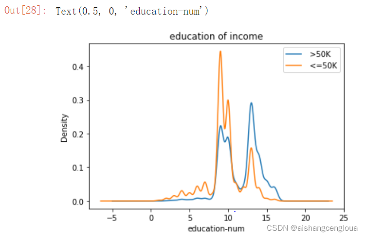

统计受教育时间对收入的影响的概率密度图。大约在时间的中值的时段，收入>50K的人是比<=50K的概率要低一些，而在中值偏右的时段是相反的，在其余时段，两种收入大约是处于平衡的状态

# fig, ([[ax1, ax2, ax3], [ax4, ax5, ax6]]) = plt.subplots(2, 3, figsize=(15, 10))
fig = plt.figure(figsize = (15, 10))

ax1 = fig.add_subplot(231) 
income_0 = df[df["race"] == ' White']["relationship"][df["income"] == 0].value_counts()
income_1 = df[df["race"] == ' White']["relationship"][df["income"] == 1].value_counts()
df1 = pd.DataFrame({' >50K' : income_1, ' <=50K' : income_0})
df1.plot(kind = 'bar', ax = ax1)
ax1.set_ylabel('number of person')
ax1.set_title('income of relationship by race_White')

ax2 = fig.add_subplot(232) 
income_0 = df[df["race"] == ' Black']["relationship"][df["income"] == 0].value_counts()
income_1 = df[df["race"] == ' Black']["relationship"][df["income"] == 1].value_counts()
df2 = pd.DataFrame({' >50K' : income_1, ' <=50K' : income_0})
df2.plot(kind = 'bar', ax = ax2)
ax2.set_ylabel('number of person')
ax2.set_title('income of relationship by race_Black')

ax3 = fig.add_subplot(233) 
income_0 = df[df["race"] == ' Asian-Pac-Islander']["relationship"][df["income"] == 0].value_counts()
income_1 = df[df["race"] == ' Asian-Pac-Islander']["relationship"][df["income"] == 1].value_counts()
df3 = pd.DataFrame({' >50K' : income_1, ' <=50K' : income_0})
df3.plot(kind = 'bar', ax = ax3)
ax3.set_ylabel('number of person')
ax3.set_title('income of relationship by race_Asian-Pac-Islander')

ax4 = fig.add_subplot(234) 
income_0 = df[df["race"] == ' Amer-Indian-Eskimo']["relationship"][df["income"] == 0].value_counts()
income_1 = df[df["race"] == ' Amer-Indian-Eskimo']["relationship"][df["income"] == 1].value_counts()
df4 = pd.DataFrame({' >50K' : income_1, ' <=50K' : income_0})
df4.plot(kind = 'bar', ax = ax4)
ax4.set_ylabel('number of person')
ax4.set_title('income of relationship by race_Amer-Indian-Eskimo')

ax5 = fig.add_subplot(235) 
income_0 = df[df["race"] == ' Other']["relationship"][df["income"] == 0].value_counts()
income_1 = df[df["race"] == ' Other']["relationship"][df["income"] == 1].value_counts()
df5 = pd.DataFrame({' >50K' : income_1, ' <=50K' : income_0})
df5.plot(kind = 'bar', ax = ax5)
ax5.set_ylabel('number of person')
ax5.set_title('income of relationship by race_Other')

plt.tight_layout()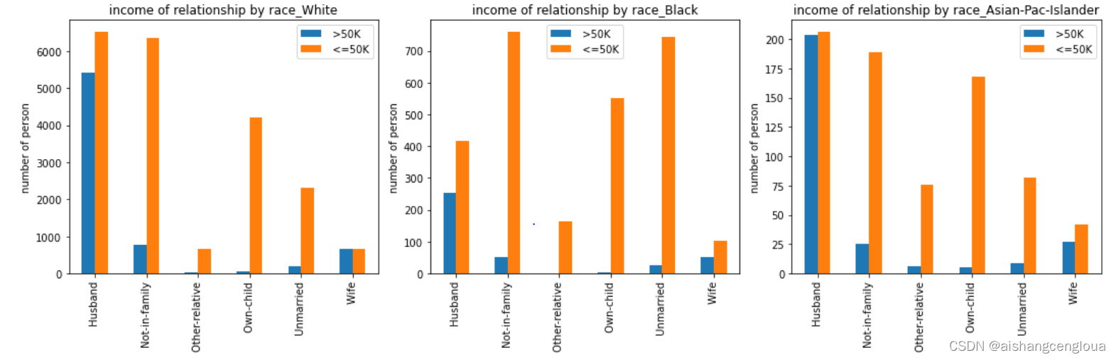

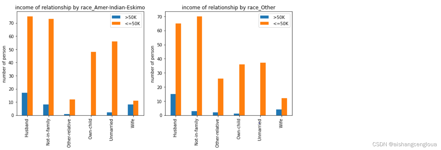
这里主要是做了不同种族扮演的社会角色的收入状况。

# fig, ([[ax1, ax2, ax3], [ax4, ax5, ax6]]) = plt.subplots(2, 3, figsize=(10, 5))
fig = plt.figure()

ax1 = fig.add_subplot(121) 
income_0 = df[df["sex"] == ' Male']["occupation"][df["income"] == 0].value_counts()
income_1 = df[df["sex"] == ' Male']["occupation"][df["income"] == 1].value_counts()
df1 = pd.DataFrame({' >50K' : income_1, ' <=50K' : income_0})
df1.plot(kind = 'bar', ax = ax1)
ax1.set_ylabel('number of person')
ax1.set_title('income of occupation by sex_Male')

ax2 = fig.add_subplot(122) 
income_0 = df[df["sex"] == ' Female']["occupation"][df["income"] == 0].value_counts()
income_1 = df[df["sex"] == ' Female']["occupation"][df["income"] == 1].value_counts()
df2 = pd.DataFrame({' >50K' : income_1, ' <=50K' : income_0})
df2.plot(kind = 'bar', ax = ax2)
ax2.set_ylabel('number of person')
ax2.set_title('income of occupation by sex_Female')

plt.tight_layout()

这里主要是做了不同性别的职业的收入状况。在男性中，职业为Exec-managerial的人中，收入>50K的人要比<=50K的人要多，而这种情况在女性中刚好相反。

df_object_col = [col for col in df.columns if df[col].dtype.name == 'object']
df_int_col = [col for col in df.columns if df[col].dtype.name != 'object' and col != 'income']
target = df["income"]
dataset = pd.concat([df[df_int_col], pd.get_dummies(df[df_object_col])], axis = 1)
dataset.head()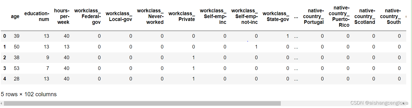

先对数据类型进行统计，对非数值型的数据进行独热编码，再将两者进行拼接。最后将收入与其他数据分开分别作为标签和训练集或者测试集

二、四种模型对上述数据集进行预测

深度学习

导入相关包

import pandas as pd 
import numpy as np
import os 
import torch
import torch.nn as nn
import torch.optim as optim
import torch.nn.functional as F
import csv
from torch.utils.tensorboard import SummaryWriter
from torch.utils.data import Dataset, DataLoader

数据预处理，要注意的是训练集和测试集进行独热编码之后可能形状不一样，所以要将他们进行配对；再者是因为我们要给缺失某列的数据进行增加全为零的列，奇怪的是当从DataFrame类型转到Numpy类型时全为零的列会全部变成nan，所以还要重新nan的列转成零。否则在预测的过程网络的输出会全部为nan。本次实验将训练集进行2 : 8的数据划分，2份作为验证集。且要对数据集进行归一化，效果会好很多

def add_missing_columns(d, columns) :
    missing_col = set(columns) - set(d.columns)
    for col in missing_col :
        d[col] = 0

def fix_columns(d, columns):  
    add_missing_columns(d, columns)
    assert(set(columns) - set(d.columns) == set())
    d = d[columns]
    return d

def data_process(df, model) :
    df.replace(" ?", pd.NaT, inplace = True)
    if model == 'train' :
        df.replace(" >50K", 1, inplace = True)
        df.replace(" <=50K", 0, inplace = True)
    if model == 'test':
        df.replace(" >50K.", 1, inplace = True)
        df.replace(" <=50K.", 0, inplace = True)

    trans = {'workclass' : df['workclass'].mode()[0], 'occupation' : df['occupation'].mode()[0], 'native-country' : df['native-country'].mode()[0]}
    df.fillna(trans, inplace = True)
    df.drop('fnlwgt', axis = 1, inplace = True)
    df.drop('capital-gain', axis = 1, inplace = True)
    df.drop('capital-loss', axis = 1, inplace = True)

    df_object_col = [col for col in df.columns if df[col].dtype.name == 'object']
    df_int_col = [col for col in df.columns if df[col].dtype.name != 'object' and col != 'income']
    target = df["income"]
    dataset = pd.concat([df[df_int_col], pd.get_dummies(df[df_object_col])], axis = 1)

    return target, dataset

class Adult_data(Dataset) :
    def __init__(self, model) :
        super(Adult_data, self).__init__()
        self.model = model

        df_train = pd.read_csv('adult.csv', header = None, names = ['age', 'workclass', 'fnlwgt', 'education', 'education-num', 'marital-status', 'occupation', 'relationship',  'race', 'sex', 'capital-gain', 'capital-loss', 'hours-per-week', 'native-country', 'income'])
        df_test = pd.read_csv('data.test', header = None, skiprows = 1, names = ['age', 'workclass', 'fnlwgt', 'education', 'education-num', 'marital-status', 'occupation', 'relationship',  'race', 'sex', 'capital-gain', 'capital-loss', 'hours-per-week', 'native-country', 'income'])

        train_target, train_dataset = data_process(df_train, 'train')
        test_target, test_dataset = data_process(df_test, 'test')

#         进行独热编码对齐
        test_dataset = fix_columns(test_dataset, train_dataset.columns)
#         print(df["income"])
        train_dataset = train_dataset.apply(lambda x : (x - x.mean()) / x.std())
        test_dataset = test_dataset.apply(lambda x : (x - x.mean()) / x.std())
#         print(train_dataset['native-country_ Holand-Netherlands'])

        train_target, test_target = np.array(train_target), np.array(test_target)
        train_dataset, test_dataset = np.array(train_dataset, dtype = np.float32), np.array(test_dataset, dtype = np.float32)
        if model == 'test' :
            isnan = np.isnan(test_dataset)
            test_dataset[np.where(isnan)] = 0.0
#             print(test_dataset[ : , 75])

        if model == 'test':
            self.target = torch.tensor(test_target, dtype = torch.int64)
            self.dataset = torch.FloatTensor(test_dataset)
        else :
#           前百分之八十的数据作为训练集，其余作为验证集
            if model == 'train' : 
                self.target = torch.tensor(train_target, dtype = torch.int64)[ : int(len(train_dataset) * 0.8)]
                self.dataset = torch.FloatTensor(train_dataset)[ : int(len(train_target) * 0.8)]
            else :
                self.target = torch.tensor(train_target, dtype = torch.int64)[int(len(train_target) * 0.8) : ] 
                self.dataset = torch.FloatTensor(train_dataset)[int(len(train_dataset) * 0.8) : ]
        print(self.dataset.shape, self.target.dtype)   

    def __getitem__(self, item) :
        return self.dataset[item], self.target[item]

    def __len__(self) :
        return len(self.dataset)

train_dataset = Adult_data(model = 'train')
val_dataset = Adult_data(model = 'val')
test_dataset = Adult_data(model = 'test')

train_loader = DataLoader(train_dataset, batch_size = 64, shuffle = True, drop_last = False)
val_loader = DataLoader(val_dataset, batch_size = 64, shuffle = False, drop_last = False)
test_loader = DataLoader(test_dataset, batch_size = 64, shuffle = False, drop_last = False)

构建网络，因为是简单的二分类，这里使用了两层感知机网络，后面做对结果进行softmax归一化。

class Adult_Model(nn.Module) :
    def __init__(self) :
        super(Adult_Model, self).__init__()
        self.net = nn.Sequential(nn.Linear(102, 64), 
                                nn.ReLU(), 
                                nn.Linear(64, 32), 
                                nn.ReLU(),
                                nn.Linear(32, 2)
                                )
    def forward(self, x) :
        out = self.net(x) 
#         print(out)
        return F.softmax(out)

训练及验证，每经过一个epoch，就进行一次损失比较，当val_loss更小时，保存最好模型，直至迭代结束。

device = torch.device('cuda' if torch.cuda.is_available() else "cpu")
model = Adult_Model().to(device)
optimizer = optim.SGD(model.parameters(), lr = 0.001, momentum = 0.9)
criterion = nn.CrossEntropyLoss()
max_epoch = 30
classes = [' <=50K', ' >50K']
mse_loss = 1000000
os.makedirs('MyModels', exist_ok = True)
writer = SummaryWriter(log_dir = 'logs')

for epoch in range(max_epoch) :

    train_loss = 0.0
    train_acc = 0.0
    model.train()
    for x, label in train_loader :
        x, label = x.to(device), label.to(device)
        optimizer.zero_grad()

        out = model(x)
        loss = criterion(out, label)
        train_loss += loss.item()
        loss.backward()

        _, pred = torch.max(out, 1)
#         print(pred)
        num_correct = (pred == label).sum().item()
        acc = num_correct / x.shape[0]
        train_acc += acc
        optimizer.step()

    print(f'epoch : {epoch + 1}, train_loss : {train_loss / len(train_loader.dataset)}, train_acc : {train_acc / len(train_loader)}')
    writer.add_scalar('train_loss', train_loss / len(train_loader.dataset), epoch)

    with torch.no_grad() :
        total_loss = []
        model.eval()
        for x, label in val_loader :
            x, label = x.to(device), label.to(device)
            out = model(x)
            loss = criterion(out, label)
            total_loss.append(loss.item())

        val_loss = sum(total_loss) / len(total_loss)

    if val_loss < mse_loss :
        mse_loss = val_loss 
        torch.save(model.state_dict(), 'MyModels/Deeplearning_Model.pth')

del model

下载在训练过程保存的最好模型进行预测并保存结果

best_model = Adult_Model().to(device)
ckpt = torch.load('MyModels/Deeplearning_Model.pth', map_location='cpu')
best_model.load_state_dict(ckpt)

test_loss = 0.0
test_acc = 0.0
best_model.eval()
result = []

for x, label in test_loader :
    x, label = x.to(device), label.to(device)

    out = best_model(x)
    loss = criterion(out, label)
    test_loss += loss.item()
    _, pred = torch.max(out, dim = 1)
    result.append(pred.detach())
    num_correct = (pred == label).sum().item()
    acc = num_correct / x.shape[0]
    test_acc += acc

print(f'test_loss : {test_loss / len(test_loader.dataset)}, test_acc : {test_acc / len(test_loader)}')

result = torch.cat(result, dim = 0).cpu().numpy()
with open('Predict/Deeplearing.csv', 'w', newline = '') as file :
    writer = csv.writer(file)
    writer.writerow(['id', 'pred_result'])
    for i, pred in enumerate(result) :
        writer.writerow([i, classes[pred]])

正确率达到0.834还是蛮不错的。

决策树

数据处理，跟深度学习的过程基本一致，只是返回值不一样而已

import pandas as pd 
import numpy as np
import csv
import graphviz
from sklearn.metrics import accuracy_score
from sklearn.model_selection import GridSearchCV
from sklearn.tree import DecisionTreeClassifier, export_graphviz

def add_missing_columns(d, columns) :
    missing_col = set(columns) - set(d.columns)
    for col in missing_col :
        d[col] = 0

def fix_columns(d, columns):  
    add_missing_columns(d, columns)
    assert(set(columns) - set(d.columns) == set())
    d = d[columns]

    return d

def data_process(df, model) :
    df.replace(" ?", pd.NaT, inplace = True)
    if model == 'train' :
        df.replace(" >50K", 1, inplace = True)
        df.replace(" <=50K", 0, inplace = True)
    if model == 'test':
        df.replace(" >50K.", 1, inplace = True)
        df.replace(" <=50K.", 0, inplace = True)
    trans = {'workclass' : df['workclass'].mode()[0], 'occupation' : df['occupation'].mode()[0], 'native-country' : df['native-country'].mode()[0]}
    df.fillna(trans, inplace = True)

    df.drop('fnlwgt', axis = 1, inplace = True)
    df.drop('capital-gain', axis = 1, inplace = True)
    df.drop('capital-loss', axis = 1, inplace = True)
#         print(df)

    df_object_col = [col for col in df.columns if df[col].dtype.name == 'object']
    df_int_col = [col for col in df.columns if df[col].dtype.name != 'object' and col != 'income']
    target = df["income"]
    dataset = pd.concat([df[df_int_col], pd.get_dummies(df[df_object_col])], axis = 1)

    return target, dataset

def Adult_data() :

    df_train = pd.read_csv('adult.csv', header = None, names = ['age', 'workclass', 'fnlwgt', 'education', 'education-num', 'marital-status', 'occupation', 'relationship',  'race', 'sex', 'capital-gain', 'capital-loss', 'hours-per-week', 'native-country', 'income'])
    df_test = pd.read_csv('data.test', header = None, skiprows = 1, names = ['age', 'workclass', 'fnlwgt', 'education', 'education-num', 'marital-status', 'occupation', 'relationship',  'race', 'sex', 'capital-gain', 'capital-loss', 'hours-per-week', 'native-country', 'income'])

    train_target, train_dataset = data_process(df_train, 'train')
    test_target, test_dataset = data_process(df_test, 'test')
#         进行独热编码对齐
    test_dataset = fix_columns(test_dataset, train_dataset.columns)
    columns = train_dataset.columns
#         print(df["income"])

    train_target, test_target = np.array(train_target), np.array(test_target)
    train_dataset, test_dataset = np.array(train_dataset), np.array(test_dataset)

    return train_dataset, train_target, test_dataset, test_target, columns

train_dataset, train_target, test_dataset, test_target, columns = Adult_data()
print(train_dataset.shape, test_dataset.shape, train_target.shape, test_target.shape)

GridSearchCV 类可以用来对分类器的指定参数值进行详尽搜索，这里搜索最佳的决策树的深度

# params = {'max_depth' : range(1, 20)}
# best_clf = GridSearchCV(DecisionTreeClassifier(criterion = 'entropy', random_state = 20), param_grid = params)
# best_clf = best_clf.fit(train_dataset, train_target)
# print(best_clf.best_params_)

用决策数进行分类，采用‘熵’作为决策基准，决策深度由上步骤得到8，分裂一个节点所需的样本数至少设为5，并保存预测结果。

# clf = DecisionTreeClassifier() score:0.7836742214851667
classes = [' <=50K', ' >50K']
clf = DecisionTreeClassifier(criterion = 'entropy', max_depth = 8, min_samples_split = 5)
clf = clf.fit(train_dataset, train_target)
pred = clf.predict(test_dataset)
print(pred)
score = clf.score(test_dataset, test_target)
# pred = clf.predict_proba(test_dataset)
print(score)
# print(np.argmax(pred, axis = 1))

with open('Predict/DecisionTree.csv', 'w', newline = '') as file :
    writer = csv.writer(file)
    writer.writerow(['id', 'result_pred'])
    for i, result in enumerate(pred) :
        writer.writerow([i, classes[result]])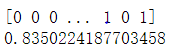

结果有0.835跟深度学习差不多
可视化决策树结构

dot_data = export_graphviz(clf, out_file = None, feature_names = columns, class_names = classes, filled = True, rounded = True)
graph = graphviz.Source(dot_data)
graph

支持向量机

因数据处理方式与决策树相同，这里不再张贴，只粘贴模型部分

from sklearn import svm
classes = [' <=50K', ' >50K']
clf = svm.SVC(kernel = 'linear')
clf = clf.fit(train_dataset, train_target)
pred = clf.predict(test_dataset)
score = clf.score(test_dataset, test_target)
print(score)
print(pred)

with open('Predict/SupportVectorMachine.csv', 'w', newline = '') as file :
    writer = csv.writer(file)
    writer.writerow(['id', 'result_pred'])
    for i, result in enumerate(pred) :
        writer.writerow([i, classes[result]])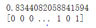

随机森林

classes = [' <=50K', ' >50K']
rf = RandomForestClassifier(n_estimators = 100, random_state = 0)
rf = rf.fit(train_dataset, train_target)
score = rf.score(test_dataset, test_target)
print(score)

pred = rf.predict(test_dataset)
print(pred)

with open('Predict/RandomForest.csv', 'w', newline = '') as file :
    writer = csv.writer(file)
    writer.writerow(['id', 'result_pred'])
    for i, result in enumerate(pred) :
        writer.writerow([i, classes[result]])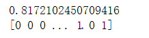

三、结果分析

经过在Adult数据集的测试集的预测结果可知，深度学习模型、决策树、支持向量机和随机森林的正确率分别达到0.834、0.834、0.834和0.817，四种模型的正确率差不多。正确率并不是很高的原因可能有：
1、模型的鲁棒性不够。
2、数据集存在大量的离散类型数据，在经过独热编码之后，数据高度稀疏。
解决方法：
1、对模型再进行搜索性地调参，可以考虑增加模型复杂度，过程中需要注意过拟合。
2、不选择独热编码的方式对数据进行降维，可以考虑Embedding

所有的代码都可以从我的 Github仓库 获取，欢迎您的start

最后，如果您对Adult数据集的处理和模型实现有收获的话，还要麻烦给点个赞，不甚感激