1 简介
短时交通流预测是实现智能交通控制与管理,交通流状态辨识和实时交通流诱导的前提及关键,也是智能化交通管理的客观需要.到目前为止,它的研究结果都不尽如人意.现有的以精确数学模型为基础的传统预测方法存在计算复杂,运算时间长,需要大量历史数据,预测精度不高等缺点.因此通过研究新型人工智能方法改进短期交通流预测具有一定的现实意义.本文在对现有短期交通流预测模型对比分析及交通流特性研究分析基础上,采用风驱动算法优化最小二乘支持向量机方法进行短期交通流预测模型,取得较好的效果. 支持向量机是一种新的机器学习算法,建立在统计学习理论的基础上,采用结构风险最小化原则,具有预测能力强,全局最优化以及收敛速度快等特点,相比较以经验风险化为基础的神经网络学习算法有更好的理论依据和更好的泛化性能.对于支持向量机模型而言,其算法相对简单,运算时间短,预测精度较高,比较适用于交通流预测研究,特别是在引入最小二乘理论后,计算简化为求解一个线性方程组,同时精度也能得到保证.,该方法首先利用风驱动算法的全局搜索能力来获取最小二乘支持向量机的惩罚因子和核函数宽度,有效解决了最小二乘支持向量机难以快速精准寻找最优参数的问题.
2 部分代码
%-------------------------------------------------------------------------
tic;
clear;
close all;
clc;
format long g;
delete('WDOoutput.txt');
delete('WDOpressure.txt');
delete('WDOposition.txt');
fid=fopen('WDOoutput.txt','a');
%--------------------------------------------------------------
% User defined WDO parameters:
param.popsize = 20;    % population size.
param.npar = 5;      % Dimension of the problem.
param.maxit = 500;    % Maximum number of iterations.
param.RT = 3;      % RT coefficient.
param.g = 0.2;      % gravitational constant.
param.alp = 0.4;    % constants in the update eq.
param.c = 0.4;      % coriolis effect.
maxV = 0.3;      % maximum allowed speed.
dimMin =  -5;      % Lower dimension boundary.
dimMax= 5;      % Upper dimension boundary.
%---------------------------------------------------------------
% Initialize WDO population, position and velocity:
% Randomize population in the range of [-1, 1]:
pos = 2*(rand(param.popsize,param.npar)-0.5);
% Randomize velocity:
vel = maxV * 2 * (rand(param.popsize,param.npar)-0.5);
%---------------------------------------------------------------
% Evaluate initial population: (Sphere Function)
for K=1:param.popsize,
  x = (dimMax - dimMin) * ((pos(K,:)+1)./2) + dimMin;
      pres(K,:) = sum (x.^2);
end
%----------------------------------------------------------------
% Finding best air parcel in the initial population :
[globalpres,indx] = min(pres);
globalpos = pos(indx,:);
minpres(1) = min(pres);      % minimum pressure
%-----------------------------------------------------------------
% Rank the air parcels:
[sorted_pres rank_ind] = sort(pres);
% Sort the air parcels:
pos = pos(rank_ind,:);
keepglob(1) = globalpres;
%-----------------------------------------------------------------
% Start iterations :
iter = 1;   % iteration counter
for ij = 2:param.maxit,
      % Update the velocity:
      for i=1:param.popsize
    % choose random dimensions:
    a = randperm(param.npar);
    % choose velocity based on random dimension:
        velot(i,:) = vel(i,a);
          vel(i,:) = (1-param.alp)*vel(i,:)-(param.g*pos(i,:))+ ...
            abs(1-1/i)*((globalpos-pos(i,:)).*param.RT)+ ...
            (param.c*velot(i,:)/i);
      end
          % Check velocity:
          vel = min(vel, maxV);
          vel = max(vel, -maxV);
    % Update air parcel positions:
        pos = pos + vel;
          pos = min(pos, 1.0);
          pos = max(pos, -1.0);
    % Evaluate population: (Pressure)
    for K=1:param.popsize,
      x = (dimMax - dimMin) * ((pos(K,:)+1)./2) + dimMin;
          pres(K,:) = sum (x.^2);
    end
      %----------------------------------------------------
      % Finding best particle in population
      [minpres,indx] = min(pres);
      minpos = pos(indx,:);             % min location for this iteration
      %----------------------------------------------------
      % Rank the air parcels:
      [sorted_pres rank_ind] = sort(pres);
      % Sort the air parcels position, velocity and pressure:
      pos = pos(rank_ind,:);
      vel = vel(rank_ind,:);
      pres = sorted_pres;
      % Updating the global best:
      better = minpres < globalpres;
      if better
            globalpres = minpres             % initialize global minimum
            globalpos = minpos;
     end
  % Keep a record of the progress:
      keepglob(ij) = globalpres;
      save WDOposition.txt pos -ascii -tabs;
end
  %Save values to the final file.
      pressure = transpose(keepglob);
      save WDOpressure.txt pressure -ascii -tabs;
        % Plot the pressure function progress over iterations:
        semilogy(keepglob, 'k' ,'LineWidth',2)
        title(['Global Best Pressure is " ',num2str(keepglob(1,param.maxit)),' ".'])
        xlabel('Number of Iterations')
        ylabel('Global Pressure (i.e. fitness) in log scale')
        grid on
        xlim([0, param.maxit])
      %END
%-----------------------------------------------------
3 仿真结果
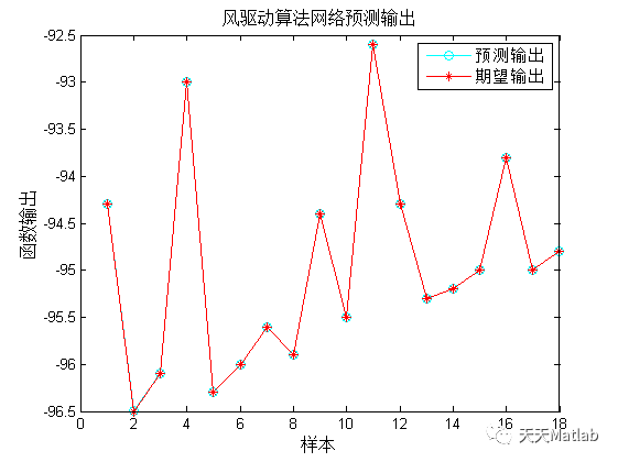
 编辑
编辑
4 参考文献
[1]刘林. 基于LSSVM的短期交通流预测研究与应用[D]. 西南交通大学, 2011.
博主简介:擅长智能优化算法、神经网络预测、信号处理、元胞自动机、图像处理、路径规划、无人机等多种领域的Matlab仿真,相关matlab代码问题可私信交流。
部分理论引用网络文献,若有侵权联系博主删除。

编辑


