1.算法仿真效果
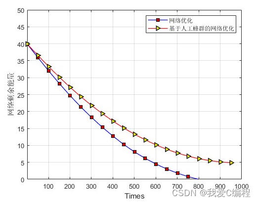
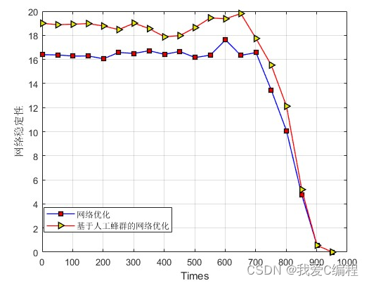
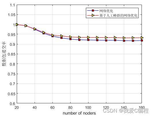
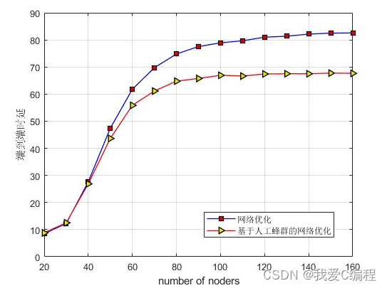
matlab2022a仿真结果如下:
2.算法涉及理论知识概要 无线传感器网络通常使用电池电源,因此能量有限,属于一次性使用。因此,无线传感器网络在原理和应用平台上都有自己的特点:
•有限的能源和存储容量
传感器节点通常布置在无人值守的运行环境中,节点能量由电池提供,但在使用过程中,电池的更换很不方便,因此无线传感器网络必须考虑如何解决能量有限的问题。因此,研究无线传感器网络优化算法以找到最大限度地减少能耗和提高无线传感器网络可靠性的最佳路径是非常重要的。
•自组织和动态拓扑结构
无线传感器网络是一种对等网络,没有严格的网络中心,生存能力强。无线传感器网络的部署不需要预先设置基础设施,传感器节点可以通过分布式算法控制行为,快速加入网络,实现自身移动,支持网络拓扑的变化。
•高容错性
当电池耗尽或环境变化时,传感器节点可能会出现故障,这将很难维护,甚至是一次性的。因此,使用优化算法来降低能耗和延长网络寿命是很重要的。
•以数据为中心
物理地址对应于传统网络节点的数据传输,传感器节点本身没有IP地址。因此,无线传感器网络只关注数据。因此,无线传感器网络是非常高效的。
•直接与物理环境互动
无线传感器网络最重要的任务是收集位置信息,这些信息需要直接与自然地理环境联系,并将现实世界的信息转换为特定的信号。因此,无线传感器网络可以单独完成数据的采样、存储、计算和发送。
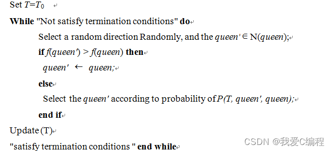
基于繁殖的人工蜂群算法包括三个步骤:蜂王的优先过程;蜂后的群集过程和幼蜂新卵的局部寻找过程。女王将把最好的基因留给下一代,因为女王基因的质量将直接决定算法的收敛速度和收敛精度。为了提高搜索效率,有必要选择最佳的女王基因。根据参考文献,采用模拟退火方法选择了蜂王基因的优先处理。根据模拟退火算法的思想,搜索过程如下:
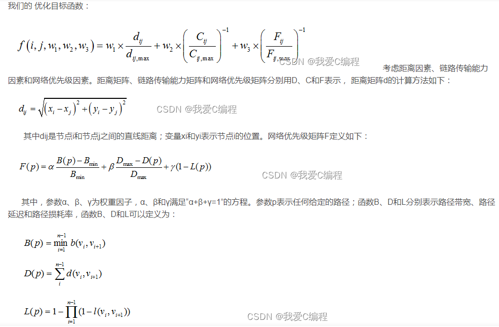
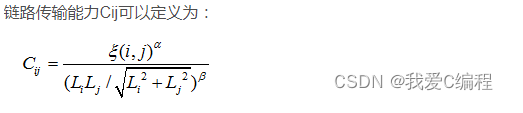
其中参数和为预设索引,α、β满足“α+β=1”的方程。参数Li和Lj分别表示节点i和节点j之间的节点自由度值。根据公式4.3,我们可以得到链路质量条件。
3.MATLAB核心程序
dmatrix= zeros(Nnode,Nnode);
matrix = zeros(Nnode,Nnode);
Trust  = zeros(Nnode,Nnode);
for i = 1:Nnode
    for j = 1:Nnode
        Dist = sqrt((X(i) - X(j))^2 + (Y(i) - Y(j))^2);
        %a link;
        if Dist <= Radius
           matrix(i,j)  = 1;
           Trust(i,j)   = 1-((T(i)+T(j))/2);
           dmatrix(i,j) = Dist;
        else
           matrix(i,j)  = inf;
           Trust(i,j)   = inf;
           dmatrix(i,j) = inf;
        end;
    end;
end;
pathS  = 1;
pathE  = Nnode;


.......................................................................

%Get the best weight
w1s=cpop(1,1);
w2s=cpop(1,2);
w1 = w1s/(w1s + w2s);
w2 = w2s/(w1s + w2s);
%%%%%%%%%%%%%%%%%%%%%%%%%%%%%%%%%%%%%%%%%%%%%%%%%%%%%%%%%%%%%%%%%%%%%%%%%%%%%

for ni = 1:length(Nnodes);
    ni
    %节点个数
    Nnode = Nnodes(ni);

    Delays2 = zeros(1,MTKL);%end-to-end delay
    consmp2 = zeros(1,MTKL);%Network topology control overhead
    Srate2  = zeros(1,MTKL);%Packet delivery rate

    for jn = 1:MTKL
        X = rand(1,Nnode)*SCALE;
        Y = rand(1,Nnode)*SCALE;
        T = rand(1,Nnode);
        Delays = zeros(Times,1);
        consmp = zeros(Times,1);
        Srate  = zeros(Times,1);
        for t = 1:Times
            if t == 1
               X = X;
               Y = Y;
            else
               %Nodes send random moves
               X = X + Vmax*rand;
               Y = Y + Vmax*rand;
            end
            %network topology
            dmatrix= zeros(Nnode,Nnode);
            matrix = zeros(Nnode,Nnode);
            Trust  = zeros(Nnode,Nnode);
            for i = 1:Nnode
                for j = 1:Nnode
                    Dist = sqrt((X(i) - X(j))^2 + (Y(i) - Y(j))^2);
                    %a link;
                    if Dist <= Radius
                       matrix(i,j)  = 1;
                       Trust(i,j)   = 1-((T(i)+T(j))/2);
                       dmatrix(i,j) = Dist;
                    else
                       matrix(i,j)  = inf;
                       Trust(i,j)   = inf;
                       dmatrix(i,j) = inf;
                    end;
                end;
            end;
            %Defines the communication start node and termination node
            tmp = randperm(Nnode);
            for i = 1:Nnode
                distA(i) = sqrt((X(i))^2 + (Y(i))^2);
                distB(i) = sqrt((X(i)-SCALE)^2 + (Y(i)-SCALE)^2);
            end
            [Va,Ia] = min(distA);
            [Vb,Ib] = min(distB);
            Sn  = Ia;
            En  = Ib;
            [paths,costs] = func_dijkstra_BF(Sn,En,dmatrix,Trust,w1,w2);
            path_distance=min(Va,Vb);
            for d=2:length(paths)
                path_distance= path_distance + dmatrix(paths(d-1),paths(d));
            end
            %end-to-end delay
            path_hops = min(length(paths)-1,1);
            %The delay is calculated based on distance, packet length, and data packet rate
            Delays(t) = path_distance*(SLen/Smax)/1e3;
            %%%%%%%%%%%%%%%%%%%%%%%%%%%%%%%%%%%%%%%%%%%%%%%%%%%%%%%%%%%%%%%
            %Packet delivery rate
            Ps       = rand/5;
            tmps     = 0;
            for ii = 1:path_hops
                tmps = tmps + path_distance*Ps^ii/1e3;
            end
            Srate(t) = 1-tmps;
            %%%%%%%%%%%%%%%%%%%%%%%%%%%%%%%%%%%%%%%%%%%%%%%%%%%%%%%%%%%%%%%
            %Network topology control overhead
            consmp(t)= 1000*path_distance*(Eelec+Eelec+Efs);
            %%%%%%%%%%%%%%%%%%%%%%%%%%%%%%%%%%%%%%%%%%%%%%%%%%%%%%%%%%%%%%%
        end
        Delays2(jn) = mean(Delays);
        Srate2(jn)  = mean(Srate);
        consmp2(jn) = mean(consmp);
    end
    ind1         = find(Delays2 > 1e5);
    ind2         = find(Delays2 < 0);
    ind          = unique([ind1,ind2]);
    Delays2(ind) = [];
    Delayn(ni)   = mean(Delays2);

    ind1         = find(Srate2 > 1);
    Srate2(ind1) = [];
    Sraten(ni)   = mean(Srate2);
    ind1         = find(consmp2 < 0);
    consmp2(ind1)= [];
    consmpn(ni)  = mean(consmp2);
end


figure;
for i = 1:Nnode
    plot(X(i),Y(i), 'ro');
    text(X(i),Y(i), num2str(i));
    hold on
end
for i = 1:length(paths)-1
    line([X(paths(i)) X(paths(i+1))], [Y(paths(i)) Y(paths(i+1))], 'LineStyle', '-');
    hold on
end

figure;
plot(Nnodes,Delayn,'b-o');
grid on
xlabel('number of noders');
ylabel('End-To-End delay');
axis([Nnodes(1),Nnodes(end),0,120]);

figure;
plot(Nnodes,Sraten,'b-o');
grid on
xlabel('number of noders');
ylabel('Packet delivery rate');
axis([Nnodes(1),Nnodes(end),0.8,1.05]);

figure;
plot(Nnodes,consmpn,'b-o');
grid on
xlabel('number of noders');
ylabel('Energy consumption');
axis([Nnodes(1),Nnodes(end),0,0.1]);


save R_new1.mat Nnodes Delayn Sraten consmpn


