1 内容介绍
物联网实现人和物的连接,感知和采集数据的无线传感器网络(Wireless Sensor Networks, WSNs)是其感知事物的核心技术.随着无线传感器网络的普及和研究的深入,基于确定性环境的假设前提,开展资源有限网络路由问题的研究难以满足实际应用的需求.无线传感器网络在部署环境,无线通信,服务质量和网络拓扑等方面同时存在众多不确定性,既有刻画事件发生与否的随机性,也有刻画对事件主观认识的模糊性.在不确定网络环境下研究无线传感器网络的路由问题,需要相应的不确定性理论和优化理论来刻画路由过程中的各种不确定因素,包括干扰模型,传播模型,移动模型和服务质量等,从而为不确定环境下WSN路由算法的研究提供理论基础和保证. 为了刻画WSN路由的不确定性,论文基于概率论,模糊集理论,模糊随机理论和优化理论进行路由模型的建模,重点对无线干扰,网络模型,服务质量和路由优化模型的不确定性进行分析和表示,同时设计相应的路由算法和仿真实验开展不确定环境下WSN路由算法的研究.
2 仿真代码
clc;
clear all;
close all;
global Qk ax ay Dik tou beta indA indB
%% Intialization
Nnodes=1;
Emax=1000;
Emin=5;
nk=8;
V=20;
%Z =[1 0.1 0.6 0.8 0.6 0 0.1 1 1 1];
%plotting network topology
%i2=1;
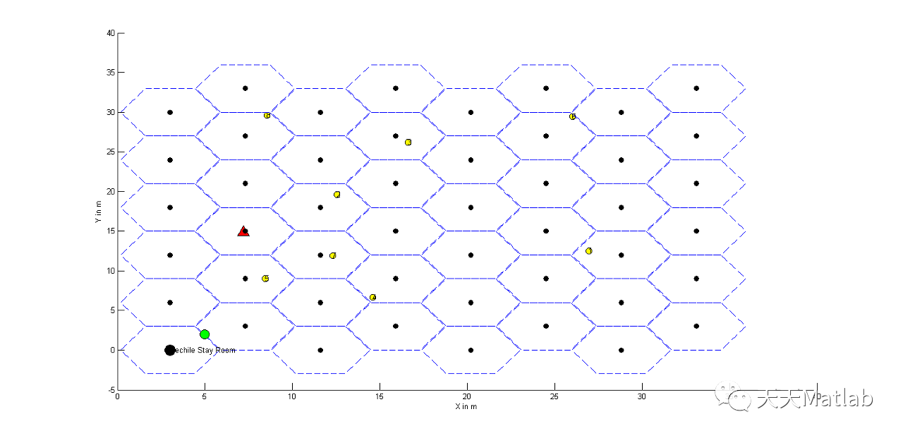
for i2 = 1:noOfNodes
plot(X(i2),Y(i2),'o','LineWidth',1,...
'MarkerEdgeColor','k',...
'MarkerFaceColor','y',...
'MarkerSize',8');
xlabel('X in m')
ylabel('Y in m')
text(X(i2), Y(i2), num2str(i2),'FontSize',10);
%% Destination
plot(X2,Y2,'^','LineWidth',1,...
'MarkerEdgeColor','k',...
'MarkerFaceColor','r',...
'MarkerSize',14');
hold on
end
axis([0 40 -5 40])
M_max = 14; %// number of cells in vertical direction
N_max = 10; %// number of cells in horizontal direction
trans = 1; %// hexagon orientation (0 or 1)
%// Do the plotting:
hold on
C11={};
C={};
ab=1;
ik=1;
for x=0:7%:2;
ik=x;
for y=0:5
if(mod(ik,2))
x0=3+4.3*x;
y0=3+3*2*y;
hexagon(2,x0,y0);
C11{x+1,y+1}=[x0;y0];
% C{ab}=[x0;y0];
hold on
plot(x0,y0,'ok','MarkerFaceColor','k')
cote=2;
x1=cote*sqrt(2)*[-1 -0.5 0.5 1 0.5 -0.5 -1]+x0;
y1=cote*sqrt(9)*[0 -0.5 -0.5 0 0.5 0.5 0]+y0;
else
x0=3+4.3*x;
y0=3*2*y;
hexagon(2,x0,y0);
C11{x+1,y+1}=[3+4.3*x;3*2*y];
hold on
plot(3+4.3*x,3*2*y,'ok', 'MarkerFaceColor','k')
cote=2;
x1=cote*sqrt(2)*[-1 -0.5 0.5 1 0.5 -0.5 -1]+x0;
y1=cote*sqrt(9)*[0 -0.5 -0.5 0 0.5 0.5 0]+y0;
end
C{ab}=[x0,y0];
%% Inside the polygon or not
[in,on] = inpolygon(X,Y,x1,y1);
Nk(ab)=numel(find(in==1));% set of sensor node
ind=[];
ind=find(in==1);
if(isempty(ind))
Dik{ab}=0;
Qk(ab)=0;
else
Dik{ab}=sqrt((X(ind)-x0).^2 +(Y(ind)-y0).^2 ); % distance froom node i to its cell center
Qk(ab)=1;
end
%Tk --> Time stays of WCV
ab=ab+1;
end
end
% axis([0 30 0 30])
% grid
%% Travelling path Model
k=ab-1;
Z=ones(1,k); %% important
aa=cell2mat(C.');
Xa=aa(:,1);
Ya=aa(:,2);
%% WCV
plot(Xa(1)+2,Ya(1)+2,'o','LineWidth',1,...
'MarkerEdgeColor','k',...
'MarkerFaceColor','g',...
'MarkerSize',12');
plot(Xa(1),Ya(1),'o','LineWidth',1,...
'MarkerEdgeColor','k',...
'MarkerFaceColor','k',...
'MarkerSize',14');
xlabel('X in m')
ylabel('Y in m')
hold on
text(Xa(1), Ya(1),'Vechile Stay Room','FontSize',10);
hold on
saveas(gcf,'fileint.fig','fig')
% %% Existing Routing
s=cell2mat(C.');
ax=s(:,1);
ay=s(:,2);
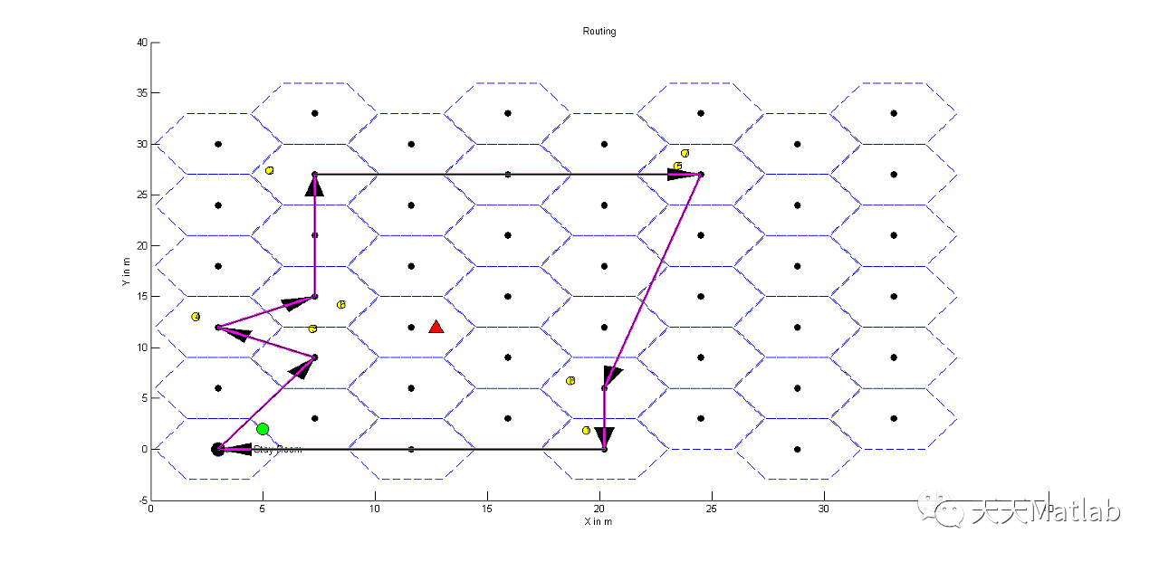
%% Routing
indA=find(Qk==1);
indB=find(Qk~=1);
G=randperm(numel(indA));
path1 = indA(G);
%% OPTIMIZATION
% %% Problem Definition
CostFunction=@(x) Sphere(x); % Cost Function
ik=1;
%cost1=1000;
eff1=inf;
while(ik<=4000)
T1=1000.*rand(1);
T=CostFunction(T1);
eff=(T);
if(eff<=eff1)
eff1=eff;
TT=T1;
end
costh1(ik)=eff1;
costh(ik)=eff;
ik=ik+1;
end
figure,
plot(1:ik-1,costh1,'-r')
hold on
plot(1:ik-1,costh,'-b')
xlabel('Iteration')
ylabel('Objective Function')
legend('Optimal','Current')
%%%%%%%%%%%%%%%%%%%%%%%
s=cell2mat(C.');
ax=s(:,1);
ay=s(:,2);
%% Routing
%rand('seed',round(TT))
s = RandStream('mt19937ar','Seed',round(TT));
G=randperm(s,numel(indA));
% G=randperm(numel(indA));
path1 = indA(G);
if(min(path1)==1)
path1=path1(path1~=1);
path = [1 path1 1];
else
path = [1 path1 1];
end
%saveas(gcf,'fileint.fig','fig')
h3=openfig('fileint.fig','new','visible')
%figure(10),
hold on
for p =1:(length(path)-1)
%line([ax(sor) ax(path(1))],[ay(sor) ay(path(1))],'Color','r','LineWidth', 1, 'LineStyle', '-')
line([ax(path(p)) ax(path(p+1))], [ay(path(p)) ay(path(p+1))], 'Color','m','LineWidth',2.5, 'LineStyle','-')
arrow([ax(path(p)) ay(path(p)) ], [ax(path(p+1)) ay(path(p+1)) ])
end
title('Routing')
%% Mathematical calc
for ab=1:numel(path)-1
dist(ab)=sqrt(((ay(path(ab))-ay(path(ab+1)))^2)+(ax(path(ab))-ax(path(ab+1)))^2);
end
L=sum(dist) % length of path
fprintf('Length is--->%3.2f\n',L)
NumJunction=numel(path);
% Distance4 bw node and chaerger
for ic=1:numel(Dik)
d(ic)=mean(Dik{ic});
end
% d=cell2mat(Dik); %--- Modified
Prx=@(d)(tou./(d+beta).^2)
Prx(d)
% Tx power of Charger
%% eqn 2
HArE=Prx;
%rand('seed',1)
deplrate=0.000001.*rand(1,numel(C)); % Nearest to sink have high depletion rate
alpha=4; % max accel/deaccel
%% single node arbitary
% Temporal Disrtize
delT=2;
fmax=1./delT;
%% Spatial node
Pmax=4;
Pmin=1;
eta1=0.5;
Cq=abs(log(Pmax/Pmin)./(log(1+eta1)))
g=1+(Cq-1).*rand(1,3); % 3 discretize space value
Pq=Pmax.*(1+eta1).^-g;
saveas(gcf,'filePr.fig','fig')
%%%%%%%%%%%%%%%%%%%%
ik=1;
%cost1=1000;
eff=0;
Ui=1000;
while(ik<=500)
[Vel,v] = randfixedsum((NumJunction).*3,1,L,0,10);
dist1=[0 dist];
for ib=1:numel(path)
rx1{ib}=Prx(d(path(ib))).*(dist1(ib)./Vel(((ib-1)*3+1):(ib*3)))-deplrate(path(ib)).*T ;% Temporal
Pqrx2{ib}=(Pq./d(path(ib)));% spatial
end
%end
Ac=cell2mat(Pqrx2);
Ac(isinf(Ac))=0;
Ad=cell2mat(rx1);
eff1=sum(Ac(:)+Ad(:));
costh21(ik)=eff1;
costh2(ik)=eff;
if(eff1>=eff)
eff=eff1;
Velb=Vel;
Ps=Pqrx2;
end
ik=ik+1;
end
figure,
plot(1:ik-1,costh21,'-r')
hold on
plot(1:ik-1,costh2,'-b')
xlabel('Iteration')
ylabel('Objective Function')
legend('Current','Optimal')
p1=cell2mat(Ps);
p1(isinf(p1))=0;
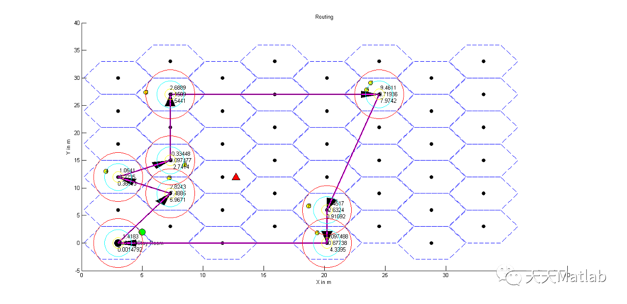
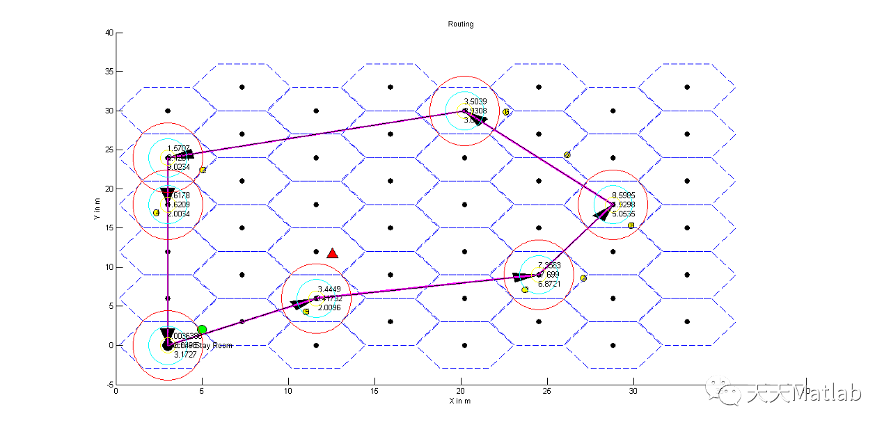
h2=openfig('filePr.fig','new','visible')
hold on
for p =1:(length(path))
if(p>=2)
text(ax(path(p)),ay(path(p)),num2str([Velb(((p-1)*3+1):(p*3))]),'FontSize',10);
%plot(ax(path(p)),ay(path(p)),'yo','MarkerSize',20)
end
if(p>=2)
plot(ax(path(p)),ay(path(p)),'yo','MarkerSize',20)
hold on
plot(ax(path(p)),ay(path(p)),'co','MarkerSize',50)
hold on
plot(ax(path(p)),ay(path(p)),'ro','MarkerSize',90)
end
hold on
end
clear path1;
clear Qk C Dik
pause(1)
end
3 运行结果
4 参考文献
[1]金劲. 群集智能算法在网络策略中的研究及其应用[D]. 兰州理工大学.
[2]王永恒, WANG, Yong-heng,等. 基于改进蚁群算法的计算机网络路由优化研究[J]. 电子设计工程, 2017(20):4.


