- 🍨 本文为🔗365天深度学习训练营 中的学习记录博客
- 🍦 参考文章地址: 365天深度学习训练营-第P6周:好莱坞明星识别
- 🍖 作者:K同学啊
一、前期准备
1.设置GPU
import torch
from torch import nn
import torchvision
from torchvision import transforms,datasets,models
import matplotlib.pyplot as plt
import os,PIL,pathlib
device = torch.device("cuda" if torch.cuda.is_available() else "cpu")
devicedevice(type='cuda')
2.导入数据
data_dir = './hlw/'
data_dir = pathlib.Path(data_dir)

data_paths = list(data_dir.glob('*'))
classNames = [str(path).split('\\')[1] for path in data_paths]
classNames
['Angelina Jolie', 'Brad Pitt', 'Denzel Washington', 'Hugh Jackman', 'Jennifer Lawrence', 'Johnny Depp', 'Kate Winslet', 'Leonardo DiCaprio', 'Megan Fox', 'Natalie Portman', 'Nicole Kidman', 'Robert Downey Jr', 'Sandra Bullock', 'Scarlett Johansson', 'Tom Cruise', 'Tom Hanks', 'Will Smith']
train_transforms = transforms.Compose([
    transforms.Resize([224,224]),# resize输入图片
    transforms.ToTensor(), # 将PIL Image或numpy.ndarray转换成tensor
    transforms.Normalize(
        mean = [0.485, 0.456, 0.406],
        std = [0.229,0.224,0.225]) # 从数据集中随机抽样计算得到
])

total_data = datasets.ImageFolder(data_dir,transform=train_transforms)
total_data
Dataset ImageFolder
Number of datapoints: 1800
Root location: hlw
StandardTransform
Transform: Compose(
Resize(size=[224, 224], interpolation=PIL.Image.BILINEAR)
ToTensor()
Normalize(mean=[0.485, 0.456, 0.406], std=[0.229, 0.224, 0.225])
)
3.数据集划分
train_size = int(0.8*len(total_data))
test_size = len(total_data) - train_size
train_dataset, test_dataset = torch.utils.data.random_split(total_data,[train_size,test_size])
train_dataset,test_dataset
(<torch.utils.data.dataset.Subset at 0x12f8aceda00>, <torch.utils.data.dataset.Subset at 0x12f8acedac0>)
train_size,test_size(1440, 360)
batch_size = 32
train_dl = torch.utils.data.DataLoader(train_dataset,
                                       batch_size=batch_size,
                                       shuffle=True,
                                       num_workers=1)
test_dl = torch.utils.data.DataLoader(test_dataset,
                                       batch_size=batch_size,
                                       shuffle=True,
                                       num_workers=1)
4. 数据可视化
imgs, labels = next(iter(train_dl))
imgs.shape
torch.Size([32, 3, 224, 224])
import numpy as np

 # 指定图片大小,图像大小为20宽、5高的绘图(单位为英寸inch)
plt.figure(figsize=(20, 5))
for i, imgs in enumerate(imgs[:20]):
    npimg = imgs.numpy().transpose((1,2,0))
    npimg = npimg * np.array((0.229, 0.224, 0.225)) + np.array((0.485, 0.456, 0.406))
    npimg = npimg.clip(0, 1)
    # 将整个figure分成2行10列,绘制第i+1个子图。
    plt.subplot(2, 10, i+1)
    plt.imshow(npimg)
    plt.axis('off')
for X,y in test_dl:
    print('Shape of X [N, C, H, W]:', X.shape)
    print('Shape of y:', y.shape)
    break
Shape of X [N, C, H, W]: torch.Size([32, 3, 224, 224]) Shape of y: torch.Size([32])
二、构建简单的CNN网络
from torchvision.models import vgg16

model = vgg16(pretrained = True).to(device)
for param in model.parameters():
    param.requires_grad = False

model.classifier._modules['6'] = nn.Linear(4096,len(classNames))

model.to(device)
model
VGG(
(features): Sequential(
(0): Conv2d(3, 64, kernel_size=(3, 3), stride=(1, 1), padding=(1, 1))
(1): ReLU(inplace=True)
(2): Conv2d(64, 64, kernel_size=(3, 3), stride=(1, 1), padding=(1, 1))
(3): ReLU(inplace=True)
(4): MaxPool2d(kernel_size=2, stride=2, padding=0, dilation=1, ceil_mode=False)
(5): Conv2d(64, 128, kernel_size=(3, 3), stride=(1, 1), padding=(1, 1))
(6): ReLU(inplace=True)
(7): Conv2d(128, 128, kernel_size=(3, 3), stride=(1, 1), padding=(1, 1))
(8): ReLU(inplace=True)
(9): MaxPool2d(kernel_size=2, stride=2, padding=0, dilation=1, ceil_mode=False)
(10): Conv2d(128, 256, kernel_size=(3, 3), stride=(1, 1), padding=(1, 1))
(11): ReLU(inplace=True)
(12): Conv2d(256, 256, kernel_size=(3, 3), stride=(1, 1), padding=(1, 1))
(13): ReLU(inplace=True)
(14): Conv2d(256, 256, kernel_size=(3, 3), stride=(1, 1), padding=(1, 1))
(15): ReLU(inplace=True)
(16): MaxPool2d(kernel_size=2, stride=2, padding=0, dilation=1, ceil_mode=False)
(17): Conv2d(256, 512, kernel_size=(3, 3), stride=(1, 1), padding=(1, 1))
(18): ReLU(inplace=True)
(19): Conv2d(512, 512, kernel_size=(3, 3), stride=(1, 1), padding=(1, 1))
(20): ReLU(inplace=True)
(21): Conv2d(512, 512, kernel_size=(3, 3), stride=(1, 1), padding=(1, 1))
(22): ReLU(inplace=True)
(23): MaxPool2d(kernel_size=2, stride=2, padding=0, dilation=1, ceil_mode=False)
(24): Conv2d(512, 512, kernel_size=(3, 3), stride=(1, 1), padding=(1, 1))
(25): ReLU(inplace=True)
(26): Conv2d(512, 512, kernel_size=(3, 3), stride=(1, 1), padding=(1, 1))
(27): ReLU(inplace=True)
(28): Conv2d(512, 512, kernel_size=(3, 3), stride=(1, 1), padding=(1, 1))
(29): ReLU(inplace=True)
(30): MaxPool2d(kernel_size=2, stride=2, padding=0, dilation=1, ceil_mode=False)
)
(avgpool): AdaptiveAvgPool2d(output_size=(7, 7))
(classifier): Sequential(
(0): Linear(in_features=25088, out_features=4096, bias=True)
(1): ReLU(inplace=True)
(2): Dropout(p=0.5, inplace=False)
(3): Linear(in_features=4096, out_features=4096, bias=True)
(4): ReLU(inplace=True)
(5): Dropout(p=0.5, inplace=False)
(6): Linear(in_features=4096, out_features=17, bias=True)
)
)
# 查看要训练的层
params_to_update = model.parameters()
# params_to_update = []
for name,param in model.named_parameters():
    if param.requires_grad == True:
#         params_to_update.append(param)
        print("\t",name)
三、训练模型
1.优化器设置
# 优化器设置
optimizer = torch.optim.Adam(params_to_update, lr=1e-4)#要训练什么参数/
scheduler = torch.optim.lr_scheduler.StepLR(optimizer, step_size=5, gamma=0.92)#学习率每5个epoch衰减成原来的1/10
loss_fn = nn.CrossEntropyLoss()
2.编写训练函数
# 训练循环
def train(dataloader, model, loss_fn, optimizer):
    size = len(dataloader.dataset)  # 训练集的大小,一共900张图片
    num_batches = len(dataloader)   # 批次数目,29(900/32)

    train_loss, train_acc = 0, 0  # 初始化训练损失和正确率

    for X, y in dataloader:  # 获取图片及其标签
        X, y = X.to(device), y.to(device)

        # 计算预测误差
        pred = model(X)          # 网络输出
        loss = loss_fn(pred, y)  # 计算网络输出和真实值之间的差距,targets为真实值,计算二者差值即为损失

        # 反向传播
        optimizer.zero_grad()  # grad属性归零
        loss.backward()        # 反向传播
        optimizer.step()       # 每一步自动更新

        # 记录acc与loss
        train_acc  += (pred.argmax(1) == y).type(torch.float).sum().item()
        train_loss += loss.item()

    train_acc  /= size
    train_loss /= num_batches

    return train_acc, train_loss
3.编写测试函数
def test (dataloader, model, loss_fn):
    size        = len(dataloader.dataset)  # 测试集的大小,一共10000张图片
    num_batches = len(dataloader)          # 批次数目,8(255/32=8,向上取整)
    test_loss, test_acc = 0, 0

    # 当不进行训练时,停止梯度更新,节省计算内存消耗
    with torch.no_grad():
        for imgs, target in dataloader:
            imgs, target = imgs.to(device), target.to(device)

            # 计算loss
            target_pred = model(imgs)
            loss        = loss_fn(target_pred, target)

            test_loss += loss.item()
            test_acc  += (target_pred.argmax(1) == target).type(torch.float).sum().item()

    test_acc  /= size
    test_loss /= num_batches

    return test_acc, test_loss
4、正式训练
训练输出层
epochs     = 20
train_loss = []
train_acc  = []
test_loss  = []
test_acc   = []
best_acc = 0
filename='checkpoint.pth'

for epoch in range(epochs):
    model.train()
    epoch_train_acc, epoch_train_loss = train(train_dl, model, loss_fn, optimizer)

    scheduler.step()#学习率衰减

    model.eval()
    epoch_test_acc, epoch_test_loss = test(test_dl, model, loss_fn)

    # 保存最优模型
    if epoch_test_acc > best_acc:
        best_acc = epoch_train_acc
        state = {
            'state_dict': model.state_dict(),#字典里key就是各层的名字,值就是训练好的权重
            'best_acc': best_acc,
            'optimizer' : optimizer.state_dict(),
        }
        torch.save(state, filename)


    train_acc.append(epoch_train_acc)
    train_loss.append(epoch_train_loss)
    test_acc.append(epoch_test_acc)
    test_loss.append(epoch_test_loss)

    template = ('Epoch:{:2d}, Train_acc:{:.1f}%, Train_loss:{:.3f}, Test_acc:{:.1f}%,Test_loss:{:.3f}')
    print(template.format(epoch+1, epoch_train_acc*100, epoch_train_loss, epoch_test_acc*100, epoch_test_loss))
print('Done')
print('best_acc:',best_acc)
Epoch: 1, Train_acc:12.2%, Train_loss:2.701, Test_acc:13.9%,Test_loss:2.544 Epoch: 2, Train_acc:20.8%, Train_loss:2.386, Test_acc:20.6%,Test_loss:2.377 Epoch: 3, Train_acc:26.1%, Train_loss:2.228, Test_acc:22.5%,Test_loss:2.274 ... Epoch:19, Train_acc:51.6%, Train_loss:1.528, Test_acc:35.8%,Test_loss:1.864 Epoch:20, Train_acc:53.9%, Train_loss:1.499, Test_acc:35.3%,Test_loss:1.852 Done best_acc: 0.37430555555555556
继续训练所有层
for param in model.parameters():
    param.requires_grad = True

# 再继续训练所有的参数,学习率调小一点
optimizer = torch.optim.Adam(model.parameters(), lr=1e-4)
scheduler = torch.optim.lr_scheduler.StepLR(optimizer, step_size=5, gamma=0.92)

# 损失函数
criterion = nn.CrossEntropyLoss()
# 加载之前训练好的权重参数
checkpoint = torch.load(filename)
best_acc = checkpoint['best_acc']
model.load_state_dict(checkpoint['state_dict'])epochs = 20
train_loss = []
train_acc = []
test_loss = []
test_acc = []
best_acc = 0
filename='best_vgg16.pth'
for epoch in range(epochs):
model.train()
epoch_train_acc, epoch_train_loss = train(train_dl, model, loss_fn, optimizer)
scheduler.step()#学习率衰减
model.eval()
epoch_test_acc, epoch_test_loss = test(test_dl, model, loss_fn)
# 保存最优模型
if epoch_test_acc > best_acc:
best_acc = epoch_test_acc
state = {
'state_dict': model.state_dict(),#字典里key就是各层的名字,值就是训练好的权重
'best_acc': best_acc,
'optimizer' : optimizer.state_dict(),
}
torch.save(state, filename)
train_acc.append(epoch_train_acc)
train_loss.append(epoch_train_loss)
test_acc.append(epoch_test_acc)
test_loss.append(epoch_test_loss)
template = ('Epoch:{:2d}, Train_acc:{:.1f}%, Train_loss:{:.3f}, Test_acc:{:.1f}%,Test_loss:{:.3f}')
print(template.format(epoch+1, epoch_train_acc*100, epoch_train_loss, epoch_test_acc*100, epoch_test_loss))
print('Done')
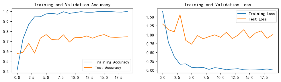
print('best_acc:',best_acc)Epoch: 1, Train_acc:41.0%, Train_loss:1.654, Test_acc:57.5%,Test_loss:1.301 Epoch: 2, Train_acc:72.3%, Train_loss:0.781, Test_acc:58.9%,Test_loss:1.139 Epoch: 3, Train_acc:87.0%, Train_loss:0.381, Test_acc:67.8%,Test_loss:1.079 ... Epoch:19, Train_acc:99.3%, Train_loss:0.033, Test_acc:74.2%,Test_loss:0.895 Epoch:20, Train_acc:99.9%, Train_loss:0.003, Test_acc:74.4%,Test_loss:1.001 Done best_acc: 0.7666666666666667
四、结果可视化
import matplotlib.pyplot as plt
#隐藏警告
import warnings
warnings.filterwarnings("ignore")               #忽略警告信息
plt.rcParams['font.sans-serif']    = ['SimHei'] # 用来正常显示中文标签
plt.rcParams['axes.unicode_minus'] = False      # 用来正常显示负号
plt.rcParams['figure.dpi']         = 100        #分辨率

epochs_range = range(epochs)

plt.figure(figsize=(12, 3))
plt.subplot(1, 2, 1)

plt.plot(epochs_range, train_acc, label='Training Accuracy')
plt.plot(epochs_range, test_acc, label='Test Accuracy')
plt.legend(loc='lower right')
plt.title('Training and Validation Accuracy')

plt.subplot(1, 2, 2)
plt.plot(epochs_range, train_loss, label='Training Loss')
plt.plot(epochs_range, test_loss, label='Test Loss')
plt.legend(loc='upper right')
plt.title('Training and Validation Loss')
plt.show()