1 简介
Matlab拟合椭圆
2 完整代码
function result = ellipseFit4HC(x,y,options)
%ellipseFit4HC Estimates the ellipse parameters, based on N pairs of
%     measured (noisy) data (x and y), together with their statistical
%     uncertainties (standard errors).
%
% SYNTAX:
%    result = ellipseFit4HC(x,y,options)
%
% INPUT:
%     x        - N-dimensional vector of x-signal measurements;
%     y        - N-dimensional vector of y-signal measurements;
%     options  - structure with the following parameters:
%              - verbose: logical variable, flag for TABLE output of the
%                estimated parameters (default value is true);
%              - isplot: logical variable, flag for graphical output
%                (default value is true);
%              - coverageFactor: coverage factor for computing the inteval
%                estimators (default value is 2);
%              - alpha: nominal significance level for computing the
%                (1-alpha)-quantiles (coverage factors) of the inteval
%                estimators (default value is alpha = [], i.e. the
%                options.coverageFactor is used);
%              - tolerance: tolerance for convergence (default is 1e-12);
%              - maxloops: maximum number of iterations (default is 100);
%              - correlation: known value of the correlation coefficient,
%                rho = corr(x,y), while assuming var(x) = var(y) = sigma2,
%                (default value is rho = 0);
%              - displconst: displacement constant (default value is
%                633.3*1000/(4*pi));
%              - displunit: displacement constant (default value is
%                picometers [pm]);
%              - smoothByFFT: smooth the original measurements (x,y)
%                by using the significant FFT frequencies.
%
% OUPUT:
%     result   - structure with detailed information on estimated
%                parameters.
%
% EXAMPLE 1: (Fit the ellipse for generated measurements x and y)
%     alpha0 = 0; beta0 = 0;        % true ellipse center [0,0]
%     alpha1 = 1; beta1 = 0.75;     % true amplitudes of x and y signals
%     phi0 = pi/3;                  % phase shift
%     X = @(t) alpha0 + alpha1 * cos(t);
%     Y = @(t) beta0 + beta1 * sin(t + phi0);
%     sigma = 0.05;                 % true measurement error STD
%     N = 50;                       % No. of observations (x,y)
%     Ncycles = 0.8;                % No. of whole ellipse cycles
%     phi = Ncycles*(2*pi)*sort(rand(N,1)); % true phases
%     x = X(phi) + sigma*randn(size(X(phi)));
%     y = Y(phi) + sigma*randn(size(Y(phi)));
%     result = ellipseFit4HC(x,y);
%
% EXAMPLE 2: (Fit the ellipse for generated measurements x and y)
%     alpha0 = 0; beta0 = 0;        % true ellipse center [0,0]
%     alpha1 = 1; beta1 = 1;        % true amplitudes
%     phi0 = pi/10;                 % phase shift
%     X = @(t) alpha0 + alpha1 * cos(t);
%     Y = @(t) beta0 + beta1 * sin(t + phi0);
%     sigma = 0.05; N = 1000; phi = (2*pi)*((1:N)')/N;
%     x = X(phi) + sigma*randn(size(X(phi)));
%     y = Y(phi) + sigma*randn(size(Y(phi)));
%     result = ellipseFit4HC(x,y)
%     disp(result.TABLE_Displacements)
%
% EXAMPLE 3: (Ellipse fit based on N = 100000 interferometer measurements)
%     load InterferometerData
%     x = data(:,1) / max(data(:,1));
%     y = data(:,2) / max(data(:,1));
%     result = ellipseFit4HC(x,y)
%     disp(result.TABLE_Displacements(1:20,:))
%
% REMARKS:
%     In particular, ellipseFit4HC can be useful for uncertaity evaluation
%     of the estimated phases and/or displacements, based on quadrature
%     homodyne interferometer measurements (with the Heydemann Correction
%     applied).
%
%     The *Heydemann Correction* is used to evaluate the phase in homodyne
%     interferometer applications to correct the interferometer
%     nonlinearities), for more details see e.g. Koening et al (2014) and
%     Wu, Su and Peng (1996).
%
%     Here we assume that the measurement errors for x and y are
%     independent (optionally correlated, with known correlation
%     coefficient rho), with zero mean and common variance sigma^2.
%
%     The standard deviation of the measurement errors, sigma, is assumed
%     to be small, such that the measurements are relatively close to the
%     true, however unobservable ellipse curve, as is the case for typical
%     interferometry measurements.
%
%     Moreover, due to numerical stability of the algorithm, it is
%     reasonable to consider normalized measurements (x,y), i.e. such that
%     the length of the main semiaxis of the fitted ellipse is close to 1.
%
%     The standard algebraic parametrization of ellipse, (A,B,C,D,E,F), see
%     e.g. Chernov & Wijewickrema (2013), is
%       A*x^2 + 2*B*x*y + C*y^2 + 2*D*x + 2*E*y + F = 0
%     or (xc,yc,a,b,alpha), in geometric parametrization of the ellipse, of
%     the following form:
%      [(x-xc)*cos(alpha) + (y-yc)*sin(alpha)]^2 / a^2 +
%         ... [(x-xc)*sin(alpha) + (y-yc)*cos(alpha)]^2 / b^2 = 1.
%     where -pi/2 < alpha < pi/2, xc, yc denote the coordinates of the
%     ellipse center, and a, b are the ellipse semiaxis.
%
%     Alternatively, one can define the ellipse also in the following
%     parametric form:
%      x(t) = xc + a * cos(t) * cos(alpha) - b * sin(t) * sin(alpha)
%      y(t) = yc + a * cos(t) * sin(alpha) + b * sin(t) * cos(alpha).
%
%     However, here we consider the following algebraic parametrization of
%     the ellipse, (B,C,D,F,G), as it is typically used in the field of
%     interferometry, see e.g. Wu, Su and Peng (1996):
%      x^2 + B*y^2 + C*x*y + D*x + F*y + G = 0,
%     and the geometric parametrization, (alpha_0,alpha_1,beta_0, beta_1,
%     phi_0) of the form:
%      x(phi) = alpha_0 + alpha_1 * cos(phi)
%      y(phi) = beta_0 + beta_1 * sin(phi + phi_0).
%     where  -pi/2 < phi0 < pi/2 is the phase offset, alpha_0, beta_0
%     denote the coordinates of the ellipse center (offsets), and alpha_1,
%     beta_1 are the signal amplitudes.
%
%     Fitting ellipse based on measurements (x,y) is a non-linear problem.
%     The presented approach is based on an approximate method which is
%     correct to the first order. It is an iterative procedure based on
%     subsequent first order Taylor expansions (linearizations) of the
%     originally nonlinear model.
%
%     The algorithm estimates the locally approximate BLUEs (Best Linear
%     Unbiased Estimators) of the ellipse parameters (B,C,D,F,G), the BLUEs
%     of the true signal values mu and nu (the values on the fitted
%     ellipse) of the measurements (x,y), together with their covariance
%     matrix, as suggested in Koening et al (2014).
%
%     This is based on iterative linearizations of the originally nonlinear
%     model with nonlinear constraints on the model parameters. For more
%     details see Kubacek (1988, p.152).
%
%     Based on that, ellipseFit4HC estimates also the geometric
%     parameters (alpha_0, alpha_1, beta_0, beta_1, phi_0) and the
%     N-dimensional vector of phases phi (and/or displacements) together
%     with their standard uncertainties computed by using the delta method.
%
% REFERENCES:
% [1] Koening, R., Wimmer, G. and Witkovsky V.: Ellipse fitting by
%     linearized nonlinear constrains to demodulate quadrature homodyne
%     interferometer signals and to determine the statistical uncertainty
%     of the interferometric phase. To appear in Measurement Science and
%     Technology, 2014.
% [2] Kubacek, L.: Foundations of Estimation Theory. Elsevier, 1988.
% [3] Chien-Ming Wu, Ching-Shen Su and Gwo-Sheng Peng. Correction of
%     nonlinearity in one-frequency optical interferometry.
%     Measurement Science and Technology, 7 (1996), 520?24.
% [4] Chernov N., Wijewickrema S.: Algorithms for projecting points onto
%     conics. Journal of Computational and Applied Mathematics 251 (2013)
%     8?1.
% (c) Viktor Witkovsky (witkovsky@savba.sk)
% Ver.: 31-Jul-2014 18:27:32
%% CHECK THE INPUTS AND OUTPUTS
tic;
narginchk(2, 3);
if nargin < 3, options = []; end
if ~isfield(options, 'smoothDataByFFT')
    options.smoothDataByFFT = false;
end
if ~isfield(options, 'displconst')
    options.displconst = 633.3*1000/(4*pi); % unit: [pm]
    %options.displconst = 633.3/(4*pi); % unit: [nm]
end
displconst = options.displconst;
if ~isfield(options, 'displunit')
    options.displunit = 'picometer [pm]';
    %options.displunit = 'nanometer [nm]';
end
displunit = options.displunit;
if ~isfield(options, 'tolerance')
    options.tolerance = 1e-12;
end
tol = options.tolerance;
if ~isfield(options, 'alpha')
    options.alpha = [];
end
if ~isfield(options, 'maxloops')
    options.maxloops = 100;
end
if ~isfield(options, 'correlation')
    options.correlation = 0;
end
if ~isfield(options, 'coverageFactor')
    options.coverageFactor = 2;
end
if ~isfield(options, 'verbose')
    options.verbose = true;
end
verbose = options.verbose;
if ~isfield(options, 'isplot')
    options.isplot = true;
end
isplot = options.isplot;
%% Initialization of the Linear model with Type II constrains
n       = length(x);
x       = x(:);
y       = y(:);
x_data  = x;
y_data  = y;
% rho is know correlation coefficient rho = corr(x,y) [default rho = 0]
% and var(x) = var(y) = sigma^2
rho = options.correlation;
% smoothDataByFFT IS EXPERIMENTAL OPTION / NOT FOR STANDARD USAGE
% Preliminary smooth the data by FFT (fit by using significant frequencies)
% This can lead to highly precise estimation of phases, if equidistant
% sampling could be reasonably assumed
if options.smoothDataByFFT
    [x,y,options] = smoothedDataByFFT(x,y,options);
end
mu_0     = x;
nu_0     = y;
if isempty(options.alpha)
    coverageFactor = options.coverageFactor;
else
    coverageFactor = tinv(1-options.alpha/2,n-5);
end
%% INITIALIZATION
B0      = [nu_0.^2, mu_0.*nu_0, mu_0, nu_0, ones(n,1)];
theta_0 = - (B0'*B0) \ (B0'*mu_0.^2);
% nonzero diagonals of A0 = [diag(A0_dg1) diag(A0_dg2)]
A0_dg1  = B0 * [0; 0; 2; theta_0(2); theta_0(3)];
A0_dg2  = B0 * [0; 0; theta_0(2); 2*theta_0(1); theta_0(4)];
c0      = mu_0.^2 + B0 * theta_0;
% Vector of observations, say Y,  Y = [x_del; y_del]
x_del   = x - mu_0;
y_del   = y - nu_0;
A0HA0_inv = sparse(1:n, 1:n, 1./(A0_dg1.^2 + A0_dg2.^2 + 2*rho*A0_dg1.*A0_dg2));
% z0 = -(c0 + A0 *[x_del;y_del]) is the right-hand side of equation
% [ A0*H*A0' B0; B0' 0] * [lambda; theta_del] = [-(c0 + A0 *[x_del;y_del]); 0]
z0       = -(c0 + A0_dg1 .* x_del + A0_dg2 .* y_del);
% Estimated parameters (1st iteration)
theta_del = (B0' * A0HA0_inv * B0) \ (B0' * A0HA0_inv * z0);
lambda    = A0HA0_inv * (z0 - B0 * theta_del);
% [mu_del; nu_del] = Y + H*A'*lambda, see Kubacek p. 152
mu_del    = x_del + (A0_dg1 + rho*A0_dg2) .* lambda;
nu_del    = y_del + (A0_dg2 + rho*A0_dg1) .* lambda;
%% ITERATIONS
maxloops  = options.maxloops;
criterion = 1;
loop      = 0;
while criterion > sqrt(n)*tol && loop < maxloops
    % LINEARIZATION:
    % Update the location (mu_0, nu_0, and theta_0) for linearization
    mu_0    = mu_0 + mu_del;
    nu_0    = nu_0 + nu_del;
    theta_0 = theta_0 + theta_del;
    % Update the measurements (x_delta, y_delta) of the linearized model
    x_del  = x - mu_0;
    y_del  = y - nu_0;
    % Update the constraints matrices (A0, B0, c0) of the linearized model
    B0     = [nu_0.^2, mu_0.*nu_0, mu_0, nu_0, ones(n,1)];
    A0_dg1 = B0 * [0; 0; 2; theta_0(2); theta_0(3)];
    A0_dg2 = B0 * [0; 0; theta_0(2); 2*theta_0(1); theta_0(4)];
    c0     = mu_0.^2 + B0 * theta_0;
    % ESTIMATION:
    % Prepare some useful matrices
    A0HA0_inv = sparse(1:n, 1:n, ...
                1./(A0_dg1.^2 + A0_dg2.^2 + 2*rho*A0_dg1.*A0_dg2));
    z0        = - (c0 + A0_dg1 .* x_del + A0_dg2 .* y_del);
    % Estimate the parameters
    theta_del = (B0' * A0HA0_inv * B0) \ (B0' * A0HA0_inv * z0);
    lambda    = A0HA0_inv * (z0 - B0 * theta_del);
    mu_del    = x_del + (A0_dg1 + rho*A0_dg2) .* lambda;
    nu_del    = y_del + (A0_dg2 + rho*A0_dg1) .* lambda;
    % CONVERGENCE: Update the value of the criterion:
    criterion = norm([mu_del; nu_del; theta_del]);
    loop      = loop + 1;
end
%% RESULTS Final estimates
% Parameters of the fitted ellipse
mu_fit       = mu_0 + mu_del;
nu_fit       = nu_0 + nu_del;
theta_fit    = theta_0 + theta_del;
% Residuals
x_res       = x_data - mu_fit;
y_res       = y_data - nu_fit;
% Residual sum of squares: sse = res' *inv(H)* res,
% where H = [I rho*I; rho*I I]
sse = (x_res' * x_res + y_res' * y_res - 2*rho* x_res' * y_res) / (1-rho^2);
% Estimated standard error
if options.smoothDataByFFT
    sigma2  = sse / (2*n-5);
else
    sigma2  = sse / (n-5);
end
sigma       = sqrt(sigma2);
% Estimated covariance matrix of the ellipse coefficients theta = (BCDFG)
theta_cov   = (B0' * A0HA0_inv * B0) \ eye(5);
theta_cov   = sigma2 * theta_cov;
theta_std   = sqrt(diag(theta_cov));
% STDs of xmean_fit and ymean_fit
[mu_std,nu_std] = munuStdFun(theta_cov,A0_dg1,A0_dg2,A0HA0_inv,B0,sigma2,rho);
% Estimated ellipse parameters (alpha0, beta0, alpha1, beta1, phi0) and their STDs
[alpha0_fit,alpha0_std] = alpha0FitFun(theta_fit,theta_cov);
[beta0_fit,beta0_std]   = beta0FitFun(theta_fit,theta_cov);
[phi0_fit,phi0_std]     = phi0FitFun(theta_fit,theta_cov);
[alpha1_fit,alpha1_std] = alpha1FitFun(theta_fit,theta_cov);
[beta1_fit,beta1_std]   = beta1FitFun(theta_fit,theta_cov);
% Estimated geometric parameters as vector
PARS_fit = [alpha0_fit;beta0_fit;alpha1_fit;beta1_fit;phi0_fit];
PARS_std = [alpha0_std;beta0_std;alpha1_std;beta1_std;phi0_std];
% Estimated phases phi_i and their STDs
[phi_fit,phi_std] = phiFitFun(mu_fit,nu_fit,theta_fit,theta_cov, ...
    A0_dg1,A0_dg2,A0HA0_inv,B0,sigma2,rho);
phi_std_max = max(phi_std);
phi_std_min = min(phi_std);
% Estimated displacements (displconst * phi_fit) and their STDs
displacement_fit = displconst * phi_fit;
displacement_std = displconst * phi_std;
% Fitted functions for x and y
X_fitfun    = @(t) alpha0_fit + alpha1_fit * cos(t);
Y_fitfun    = @(t) beta0_fit + beta1_fit * sin(t + phi0_fit);
%% TABLE Estimated ellipse parameters: (B, C, D, F, G)
TABLE_BCDFG = table;
TABLE_BCDFG.Properties.Description = ...
    'Estimated Ellipse Parameters (B,C,D,F,G)';
TABLE_BCDFG.ESTIMATE = theta_fit;
TABLE_BCDFG.STD  = theta_std;
TABLE_BCDFG.DF = (n-5)*ones(5,1);
TABLE_BCDFG.FACTOR = coverageFactor*ones(5,1);
TABLE_BCDFG.LOWER = theta_fit - coverageFactor*theta_std;
TABLE_BCDFG.UPPER = theta_fit + coverageFactor*theta_std;
TABLE_BCDFG.Properties.RowNames = {'B'  'C'  'D'  'F'  'G'};
%% TABLE Estimated ellipse parameters: (alpha0, beta0, alpha1, beta1, phi0)
TABLE_EllipsePars = table;
TABLE_EllipsePars.Properties.Description = ...
    'Estimated Ellipse Parameters (alpha_0, beta_0, alpha_1, beta_1, phi_0)';
TABLE_EllipsePars.ESTIMATE = PARS_fit;
TABLE_EllipsePars.STD  = PARS_std;
TABLE_EllipsePars.DF = (n-5)*ones(5,1);
TABLE_EllipsePars.FACTOR = coverageFactor*ones(5,1);
TABLE_EllipsePars.LOWER = PARS_fit - coverageFactor*PARS_std;
TABLE_EllipsePars.UPPER = PARS_fit + coverageFactor*PARS_std;
TABLE_EllipsePars.Properties.RowNames = ...
    {'alpha_0' 'beta_0' 'alpha_1' 'beta_1' 'phi_0'};
%% TABLE Estimated dispacements: const * phi
TABLE_Displacements = table;
TABLE_Displacements.Properties.Description = ...
    ['Estimated Displacements, ',displunit];
TABLE_Displacements.OBSERVATION = (1:n)';
TABLE_Displacements.ESTIMATE = displacement_fit;
TABLE_Displacements.STD  = displacement_std;
TABLE_Displacements.DF = (n-5)*ones(n,1);
TABLE_Displacements.FACTOR = coverageFactor*ones(n,1);
TABLE_Displacements.LOWER = ...
    displacement_fit - coverageFactor*displacement_std;
TABLE_Displacements.UPPER = ...
    displacement_fit + coverageFactor*displacement_std;
%% RESULTS / Set the result
result.Description = ...
    'Ellipse Fit by Iterated Locally Best Linear Unbiased Estimation';
% Standard Algebraic Parametrization: Ax^2 + 2Bxy + Cy^2 + 2Dx + 2Ey + F = 0
result.ABCDEF_Description = 'A*x^2 + 2*B*x*y + C*y^2 + 2*D*x + 2*E*y + F = 0';
%result.ABCDEF_VarNames = {'x.^2' '2*x.*y' 'y.^2' '2*x' '2*y' '1'};
result.ABCDEF_Names = {'A' 'B' 'C' 'D' 'E' 'F'};
result.ABCDEF_fit = [1; theta_fit(2)/2; theta_fit(1);...
    theta_fit(3)/2; theta_fit(4)/2;theta_fit(5)]';
result.ABCDEF_std = [0; theta_std(2)/2; theta_std(1);...
    theta_std(3)/2; theta_std(4)/2;theta_std(5)]';
% Algebraic Parametrization (Peng-Wu): x^2 + By^2 +  Cxy + Dx + Fy + G = 0
result.BCDFG_Description = 'x^2 + B*y^2 +  C*x*y + D*x + F*y + G = 0';
%result.BCDFG_VarNames = {'y.^2' 'x.*y' 'x' 'y' '1'};
result.BCDFG_Names = {'B' 'C' 'D' 'F' 'G'};
result.BCDFG_fit = theta_fit';
result.BCDFG_std = theta_std';
result.BCDFG_cov = theta_cov;
% Geometric Parametrization (Peng-Wu): (alpha_0, beta_0, alpha_1, beta_1, phi_0)
% X(phi) = alpha_0 + alpha_1 * cos(phi)
% Y(phi) = beta_0  + beta_1  * sin(phi + phi_0
result.EllipsePars_Description_X = 'X(phi) = alpha_0 + alpha_1 * cos(phi)';
result.EllipsePars_Description_Y = 'Y(phi) = beta_0  + beta_1  * sin(phi + phi_0)';
result.EllipsePars_Names = {'alpha_0' 'beta_0' 'alpha_1' 'beta_1' 'phi_0'};
result.EllipsePars_fit = PARS_fit';
result.EllipsePars_std = PARS_std';
% Estimated mu
result.mu_X_fit = mu_fit;
result.mu_X_std = mu_std;
% Estimated nu
result.nu_Y_fit = nu_fit;
result.nu_Y_std = nu_std;
% Fitted functions
result.X_fitfun = X_fitfun;
result.Y_fitfun = Y_fitfun;
% Estimated residuals
result.x_res_fit = x_res;
result.x_res_std = sqrt(sigma2 - mu_std.^2);
result.y_res_fit = y_res;
result.y_res_std = sqrt(sigma2 - nu_std.^2);
% Estimated sigma
result.sigma_fit = sigma;
result.sigma2_fit = sigma.^2;
% Estimated phases phi
result.phi_fit = phi_fit;
result.phi_std = phi_std;
result.phi_std_max = phi_std_max;
result.phi_std_min = phi_std_min;
%result.phi_std_mean = mean(phi_std);
% Estimated Displacements
result.Displacement_Description = ...
    'Displacement_fit = Displacement_const * phi_fit';
result.Displacement_fit = displacement_fit;
result.Displacement_std = displacement_std;
result.Displacement_std_max = displconst*phi_std_max;
result.Displacement_std_min = displconst*phi_std_min;
%result.Displacement_std_mean = displconst*mean(phi_std);
result.Displacement_const = displconst;
result.Displacement_unit = displunit;
% TABLES
result.TABLE_BCDFG = TABLE_BCDFG;
result.TABLE_EllipsePars = TABLE_EllipsePars;
result.TABLE_Displacements = TABLE_Displacements;
% Info
result.x_data = x_data;
result.y_data = y_data;
result.used_Correlation_XY = rho;
result.options = options;
result.criterion = criterion;
result.loops = loop;
result.tictoc = toc;
%% PLOT FIGURE / Fitted Ellipse
if isplot
    t = linspace(0,2*pi,1000)';
    figWidth = 1024; figHeight = 1024; % size in pixels
    rect = [10 10 figWidth figHeight];
    figure1 = figure('Name','FittedEllipse','OuterPosition', rect);
    axes1 = axes('Parent',figure1,'PlotBoxAspectRatio',...
        [1 1 1],'DataAspectRatio',[1 1 1]);
    box(axes1,'on');
    hold(axes1,'all');
    plot1 = plot(x_data,y_data,'x', ...
        alpha0_fit,beta0_fit,'h', ...
        X_fitfun(t),Y_fitfun(t),'--', ...
        mu_fit,nu_fit,'o', ...
        'LineWidth',2,'MarkerSize',8);
    set(plot1(1),'DisplayName','measurements (x,y)');
    set(plot1(2),'Color',[0 0 0],'MarkerFaceColor','g', ...
        'DisplayName','fitted ellipse center');
    set(plot1(3),'Color',[1 0 1],'DisplayName','fitted ellipse');
    set(plot1(4),'Color',[1 0 1],'MarkerFaceColor','g', ...
        'DisplayName','fitted values (X,Y)',...
        'LineWidth',1,'MarkerSize',5);
    xlabel('x');
    ylabel('y');
    legend1 = legend(axes1,'show');
    set(legend1,'Location','NorthWest');
    grid
end
%% SHOW TABLES
if verbose
    disp('  -------------------------------------------------')
    disp('  ESTIMATED ELLIPSE PARAMETERS                     ')
    disp('  X^2 + B*Y^2 + C*X*Y + D*X + F*Y + G = 0          ')
    disp('  -------------------------------------------------')
    disp(TABLE_BCDFG)
    disp('  -------------------------------------------------')
    disp('  ESTIMATED ELLIPSE PARAMETERS                     ')
    disp('  X(phi) = alpha_0 + alpha_1 * cos(phi)            ')
    disp('  Y(phi) = beta_0  + beta_1  * sin(phi + phi_0     ')
    disp('  -------------------------------------------------')
    disp(TABLE_EllipsePars)
%    disp(TABLE_Displacements)
%    disp('  -------------------------------------------------')
%    disp('  ESTIMATED DISPLACEMENTS ')
%    disp('  -------------------------------------------------')
end
%% END OF ellipseFit4HC
end
%% Function ATANVW
% function phi = atanvw(nom_y,den_x)
% %ATANVW Computes standardized value of the angle phi in interval [0,2*pi]
% %       based on arctan of nom/den.
%
% % (c) Viktor Witkovsky (witkovsky@savba.sk)
% % Ver.: 15-Sep-2013 10:40:28
%
% %% CHECK INPUTS AND OUTPUTS
% narginchk(2, 2);
%
% %%
% phi = zeros(size(nom_y));
% nomsgn = sign(nom_y);
% densgn = sign(den_x);
% tmp = (nomsgn == 1 & densgn == 1);
% phi(tmp) = atan(abs(nom_y(tmp)./den_x(tmp)));
% tmp = (nomsgn == 1 & densgn == -1);
% phi(tmp) = pi - atan(abs(nom_y(tmp)./den_x(tmp))) ;
% tmp = (nomsgn == -1 & densgn == -1);
% phi(tmp) = pi + atan(abs(nom_y(tmp)./den_x(tmp)));
% tmp = (nomsgn == -1 & densgn == 1);
% phi(tmp) = 2*pi - atan(abs(nom_y(tmp)./den_x(tmp)));
%
% end
%% Function alpha0FitFun
function [alpha0_fit,alpha0_std,alpha0_grad] = alpha0FitFun(BCDFG,BCDFG_cov)
%alpha0FitFun Computes the fitted value alpha0_fit and its uncertainty (STD),
%       based on estimated ellipse coefficients BCDFG and their
%       estimated covariance matrix BCDFG_cov.
% (c) Viktor Witkovsky (witkovsky@savba.sk)
% Ver.: 31-Jul-2014 18:27:32
% Fitted coefficients
B = BCDFG(1);
C = BCDFG(2);
D = BCDFG(3);
F = BCDFG(4);
% G = BCDFG(5);
% Fitted value of alpha0 (x-center of the ellipse)
DEN = 4*B - C^2;
alpha0_fit = (C*F - 2*B*D) / DEN;
% Gradient
alpha0_grad    = zeros(5,1);
alpha0_grad(1) = (2*C*(C*D - 2*F))/DEN^2;
alpha0_grad(2) = (C^2*F + 4*B*(-C*D + F))/DEN^2;
alpha0_grad(3) = -2*B/DEN;
alpha0_grad(4) = C/DEN;
% Standard deviation (STD)
alpha0_std = sqrt(alpha0_grad' * BCDFG_cov * alpha0_grad);
end
%% Function beta0FitFun
function [beta0_fit,beta0_std,beta0_grad] = beta0FitFun(BCDFG,BCDFG_cov)
%beta0FitFun Computes the fitted value beta0_fit and its uncertainty (STD),
%       based on estimated ellipse coefficients BCDFG and their
%       estimated covariance matrix BCDFG_cov.
% (c) Viktor Witkovsky (witkovsky@savba.sk)
% Ver.: 31-Jul-2014 18:27:32
% Fitted coefficients
B = BCDFG(1);
C = BCDFG(2);
D = BCDFG(3);
F = BCDFG(4);
% G = BCDFG(5);
% Fitted value of beta0 (y-center of the ellipse)
DEN = 4*B - C^2;
beta0_fit = (C*D - 2*F) / DEN;
% Gradient
beta0_grad    = zeros(5,1);
beta0_grad(1) = (-4*C*D + 8*F) / DEN^2;
beta0_grad(2) = (4*B*D + C*(C*D - 4*F)) / DEN^2;
beta0_grad(3) = C / DEN;
beta0_grad(4) = -2 / DEN;
% Standard deviation (STD)
beta0_std = sqrt(beta0_grad' * BCDFG_cov * beta0_grad);
end
%% Function phi0FitFun
function [phi0_fit,phi0_std,phi0_grad] = phi0FitFun(BCDFG,BCDFG_cov)
%phi0FitFun Computes the fitted value phi0_fit and its uncertainty (STD),
%       based on estimated ellipse coefficients BCDFG and their
%       estimated covariance matrix BCDFG_cov.
% (c) Viktor Witkovsky (witkovsky@savba.sk)
% Ver.: 31-Jul-2014 18:27:32
% Fitted coefficients
B = BCDFG(1);
C = BCDFG(2);
% D = BCDFG(3);
% F = BCDFG(4);
% G = BCDFG(5);
% Fitted value of phi0 (phase offset of the ellipse)
phi0_fit = asin(-C/(2*sqrt(B)));
% Gradient
DEN = sqrt(B) * sqrt(1-C^2/(4*B));
phi0_grad    = zeros(5,1);
phi0_grad(1) = -1 / (2*DEN);
phi0_grad(2) = C / (4*B*DEN);
% Standard deviation (STD)
phi0_std = sqrt(phi0_grad' * BCDFG_cov * phi0_grad);
end
%% Function alpha1FitFun
function [alpha1_fit,alpha1_std,alpha1_grad] = alpha1FitFun(BCDFG,BCDFG_cov)
%alpha1FitFun Computes the fitted value alpha1_fit and its uncertainty (STD),
%       based on estimated ellipse coefficients BCDFG and their
%       estimated covariance matrix BCDFG_cov.
% (c) Viktor Witkovsky (witkovsky@savba.sk)
% Ver.: 31-Jul-2014 18:27:32
% Fitted coefficients
B = BCDFG(1);
C = BCDFG(2);
D = BCDFG(3);
F = BCDFG(4);
G = BCDFG(5);
% Fitted value of alpha1 (x-semi-axis of the ellipse)
DEN  = 4*B - C^2;
DEN2 = sqrt(-C*D*F + F^2 + B*(D^2 - 4*G) + C^2*G);
alpha1_fit = (2*sqrt(B) * sqrt(B*D^2 - C*D*F + F^2 - (4*B - C^2)*G)) / DEN;
% Gradient
alpha1_grad = zeros(5,1);
alpha1_grad(1) = (B*(4*C*D*F - 4*F^2 - 2*C^2*(D^2 - 2*G)) - C^2* ...
    (-C*D*F + F^2 + C^2*G))/(sqrt(B)*DEN^2*DEN2);
alpha1_grad(2) = (sqrt(B)*(4*B*(-D*F + C*(D^2 - 2*G)) + C* ...
    (-3*C*D*F + 4*F^2 + 2*C^2*G)))/(DEN^2*DEN2);
alpha1_grad(3) = (sqrt(B)*(2*B*D - C*F)) /(DEN*DEN2);
alpha1_grad(4) = sqrt(B)*(-C*D + 2*F)/(DEN*DEN2);
alpha1_grad(5) = -sqrt(B) / DEN2;
% Standard deviation (STD)
alpha1_std = sqrt(alpha1_grad' * BCDFG_cov * alpha1_grad);
end
%% Function beta1FitFun
function [beta1_fit,beta1_std,beta1_grad] = beta1FitFun(BCDFG,BCDFG_cov)
%beta1FitFun Computes the fitted value beta1_fit and its uncertainty (STD),
%       based on estimated ellipse coefficients BCDFG and their
%       estimated covariance matrix BCDFG_cov.
% (c) Viktor Witkovsky (witkovsky@savba.sk)
% Ver.: 31-Jul-2014 18:27:32
% Fitted coefficients
B = BCDFG(1);
C = BCDFG(2);
D = BCDFG(3);
F = BCDFG(4);
G = BCDFG(5);
% Fitted value of beta1 (y-semi-axis of the ellipse)
DEN = 4*B - C^2;
DEN2 = sqrt(-C*D*F + F^2 + B*(D^2 - 4*G) + C^2*G);
beta1_fit = (2*sqrt(B*D^2 - C*D*F + F^2 - (4*B - C^2)*G))/DEN;
% Gradient
beta1_grad = zeros(5,1);
beta1_grad(1) = (8*C*D*F - 8*F^2 - 4*B* (D^2 - 4*G) - ...
    C^2*(D^2 + 4*G)) /(DEN^2*DEN2);
beta1_grad(2) = (4*B*(-D*F + C*(D^2 - 2*G)) + ...
    C*(-3*C*D*F + 4*F^2 + 2*C^2*G))/(DEN^2*DEN2);
beta1_grad(3) = (2*B*D - C*F) / (DEN*DEN2);
beta1_grad(4) = (-C*D + 2*F) / (DEN*DEN2);
beta1_grad(5) = -1 / DEN2;
% Standard deviation (STD)
beta1_std = sqrt(beta1_grad' * BCDFG_cov * beta1_grad);
end
%% Function phiFitFun
function [phi_fit,phi_std,phi_grad] = ...
    phiFitFun(mu,nu,BCDFG,BCDFG_cov,A0_dg1,A0_dg2,A0HA0inv,B0,sig2,rho)
%phiFitFun Computes the fitted value phi_fit and its uncertainty (STD),
%       based on estimated ellipse coefficients BCDFG and their
%       estimated covariance matrix BCDFG_cov.
% (c) Viktor Witkovsky (witkovsky@savba.sk)
% Ver.: 31-Jul-2014 18:27:32
% Fitted coefficients
B = BCDFG(1);
C = BCDFG(2);
D = BCDFG(3);
F = BCDFG(4);
% G = BCDFG(5);
% Fitted value of phase phi
n = length(mu);
nom = sqrt(4*B - C^2)*(F + C*mu + 2*B*nu);
den = (2*B*(D + 2*mu) - C*(F + C*mu));
%phi_fit = atanvw(nom,den);
phi_fit = atan2(nom,den);
% Gradient
DEN = 4*B - C^2;
DEN2 = sqrt(DEN)*(4*B^2*nu.^2 + B*((D + 2*mu).^2 + ...
    4*(F + C*mu).*nu - C^2*nu.^2) -  ...
    (F + C*mu).*(-F + C*(D + mu + C*nu)));
phi_grad = zeros(n,7);
phi_grad(:,1) = (sqrt(DEN)*(-2*(F + 2*B*nu) + ...
    C*(D + C*nu))) ./ (2*(4*B^2*nu.^2 + B*((D + 2*mu).^2 + ...
    4*(F + C*mu).*nu - C^2*nu.^2) - (F + C*mu).*(-F + C*(D + mu + C*nu))));
phi_grad(:,2) =  (2*B*sqrt(DEN)*(2*B*(D + 2*mu) - C*(F + C*mu))) ./ ...
    ((-2*B*(D + 2*mu) + C*(F + C*mu)).^2 + ...
    (4*B - C^2)*(F + C*mu + 2*B*nu).^2);
phi_grad(:,3) = (4*B^2*(D + 2*mu).*nu - ...
    2*B*(F + C*mu).*(D + 2*mu + 3*C*nu) + C*(F + C*mu).* ...
    (-F + C*(D + mu + C*nu))) ./ (2*B*DEN2);
phi_grad(:,4) = (-2*C^2*mu.*(D + mu) - C^3*mu.*nu - ...
    C*(D - 2*mu).*(F + 2*B*nu) + ...
    2*(F^2 + 2*B*mu.*(D + 2*mu) + 2*B*F*nu)) ./ (2*DEN2);
phi_grad(:,5) = (-2*B*sqrt(DEN)*(F + C*mu + 2*B*nu)) ./ ...
    ((-2*B*(D + 2*mu) + C*(F + C*mu)).^2 + ...
    (4*B - C^2)*(F + C*mu + 2*B*nu).^2);
phi_grad(:,6) = sqrt(DEN)*(D + 2*mu + C*nu) ./ ...
    (2*(4*B^2*nu.^2 + B*((D + 2*mu).^2 + 4*(F + C*mu).*nu - C^2*nu.^2) -...
    (F + C*mu).*(-F + C*(D + mu + C*nu))));
% Compute H*A' = [I rho*I; rho*I I] * [diag(A0_dg1); diag(A0_dg2)]
HA0_dg1 = A0_dg1 + rho*A0_dg2;
HA0_dg2 = A0_dg2 + rho*A0_dg1;
% B1B1inv = sparse(1:n,1:n,1./(B1_diag1.^2 + B1_diag2.^2));
A0grad = HA0_dg1.*phi_grad(:,1) + HA0_dg2.*phi_grad(:,2);
B0A0grad =  repmat(A0HA0inv * A0grad,1,5) .* B0;
% Variance (VAR) of phi_i (contributions to variance of estimator of phi_i)
% phi_var = phi_grad(:,1:2)'*Sigma_11*phi_grad(:,1:2) +
%           2*phi_grad(:,1:2)'*Sigma_12*phi_grad(:,3:end) +
%           phi_grad(:,3:end)'*Sigma_22*phi_grad(:,3:end)
phi_var = sig2*((phi_grad(:,1).^2 + phi_grad(:,2).^2) + ...
      2*rho * phi_grad(:,1) .* phi_grad(:,2) - ...
      A0grad .* (A0HA0inv*A0grad));
phi_var = phi_var + sum((B0A0grad*BCDFG_cov) .* B0A0grad,2);
phi_var = phi_var + sum((B0A0grad*BCDFG_cov) .* phi_grad(:,3:end),2);
phi_var = phi_var + sum((phi_grad(:,3:end)*BCDFG_cov).*phi_grad(:,3:end),2);
% Standard deviation (STD) of phi_i
phi_std = sqrt(phi_var);
end
%% Function munuStdFun
function [mu_std,nu_std] = ...
    munuStdFun(theta_cov,A0_dg1,A0_dg2,A0HA0_inv,B0,sigma2,rho)
%munuStdFun Computes the uncertainties (STDs), of the mu_fit and nu_fit.
% (c) Viktor Witkovsky (witkovsky@savba.sk)
% Ver.: 31-Jul-2014 18:27:32
% Compute H*A' = [I rho*I; rho*I I] * [diag(A0_dg1); diag(A0_dg2)]
HA0_dg1 = A0_dg1 + rho*A0_dg2;
HA0_dg2 = A0_dg2 + rho*A0_dg1;
HAAHAB1 =  repmat(A0HA0_inv * HA0_dg1,1,5) .* B0;
mu_std = sqrt(sigma2*(1 - HA0_dg1 .* (A0HA0_inv*HA0_dg1)) ...
    + sum((HAAHAB1*theta_cov) .* HAAHAB1,2));
HAAHAB2 =  repmat(A0HA0_inv * HA0_dg2,1,5) .* B0;
nu_std = sqrt(sigma2*(1 - HA0_dg2 .* (A0HA0_inv*HA0_dg2)) ...
    + sum((HAAHAB2*theta_cov) .* HAAHAB2,2));
end
%% Function smoothByFFT
function [xs,ys,options] = smoothedDataByFFT(x,y,options)
% smoothByFFT Smooth the original measurements (x,y) by using the
%    significant FFT frequencies
% (c) Viktor Witkovsky (witkovsky@savba.sk)
% Ver.: 22-Feb-2014 15:10:24
narginchk(2, 3);
if nargin < 3, options = []; end
if  ~isfield(options, 'fftthreshold')
    options.fftthreshold = 0.1;
end
if  ~isfield(options, 'fftsmooththreshold')
    options.fftsmooththreshold = 0.01;
end
fftthreshold = options.fftthreshold;
fftsmooththreshold = options.fftsmooththreshold;
if  ~isfield(options, 'fftindx')
    fftx = abs(fftshift(fft(x)));
    fftmaxx = max(fftx);
    fftindx1 = find(fftx >= fftmaxx *fftthreshold);
    fftindx1 = unique(sort([fftindx1;mean(fftindx1)]));
    fftindx2 = find(fftx >= fftmaxx *fftsmooththreshold);
    fftindx2 = unique(sort([fftindx2;mean(fftindx2)]));
    options.fftindx = fftindx2;
end
if  ~isfield(options, 'fftindy')
    ffty = abs(fftshift(fft(y)));
    fftmaxy = max(ffty);
    fftindy1 = find(ffty >= fftmaxy *fftthreshold);
    fftindy1 = unique(sort([fftindy1;mean(fftindy1)]));
    fftindy2 = find(ffty >= fftmaxy *fftsmooththreshold);
    fftindy2 = unique(sort([fftindy2;mean(fftindy2)]));
    options.fftindy = fftindy2;
end
indx1 = fftindx1;
indy1 = fftindy1;
xfft = fftshift(fft(x));
indX1 = setdiff(1:numel(xfft),indx1);
xfft(indX1) = 0;
xs = ifft(ifftshift(xfft));
yfft = fftshift(fft(y));
indY1 = setdiff(1:numel(yfft),indy1);
yfft(indY1) = 0;
ys = ifft(ifftshift(yfft));
end
%% ellipseFit4HC_EXAMPLE
clear
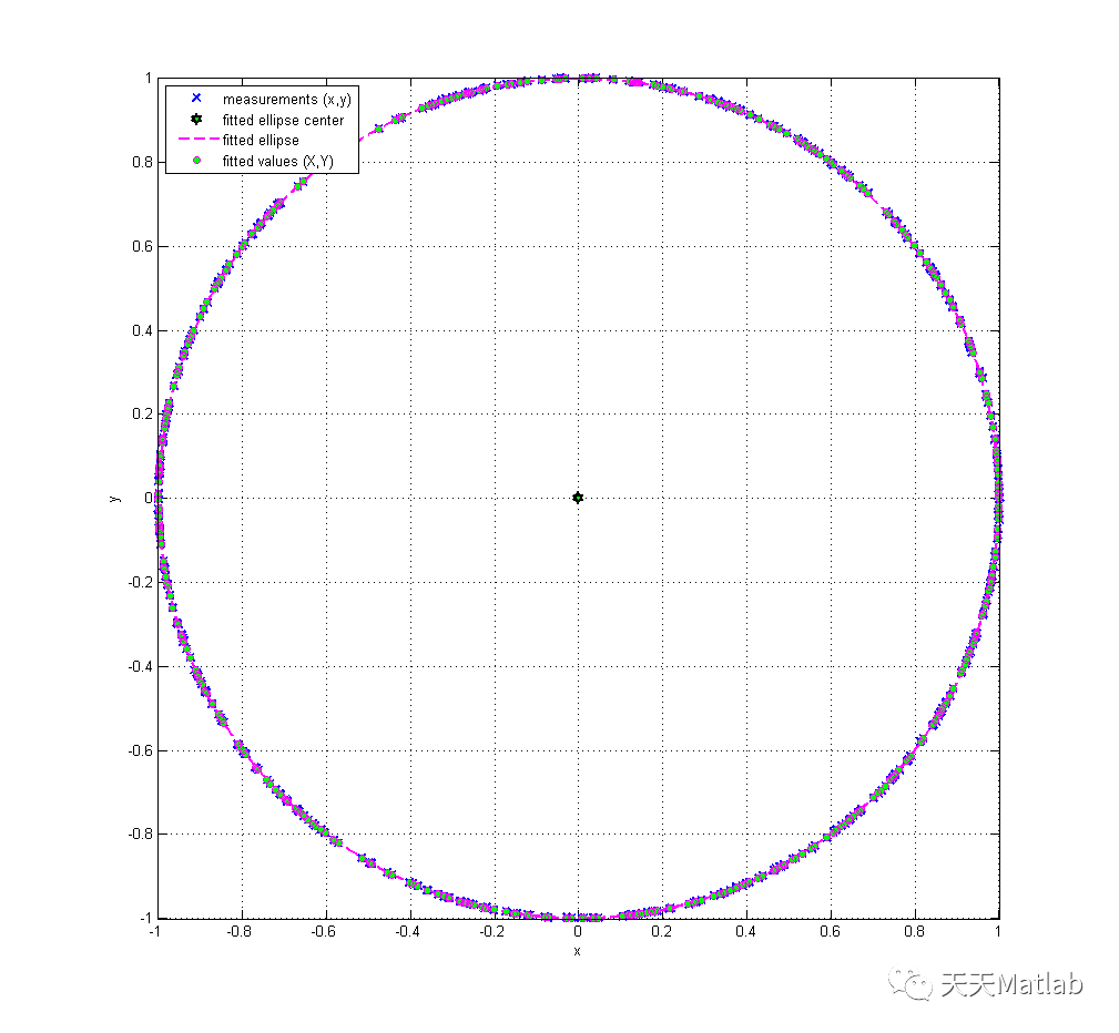
%% GENERATE the uncorrelated measurements: x and y
% Feel free to experiment with the setting parameters
alpha0true = 0; % x-center (offset x)
beta0true = 0; % y-center (offset x)
alpha1true = 1; % x-amplitude
beta1true = 1; % y-amplitude
phi0true = 0; % phase offset
sigma = 0.001; % std of x and y independent errors
n = 500; % number of measurements points
cycles = 1; % measurement interval, # cycles
phitrue = cycles*(2*pi)*sort(rand(n,1)); % true phases phi_i
% true values: X and Y
Xmean = @(t) alpha0true + alpha1true * cos(t);
Ymean = @(t) beta0true + beta1true * sin(t + phi0true);
% measurements: X + error, Y + error,
x = Xmean(phitrue) + sigma * randn(size(phitrue));
y = Ymean(phitrue) + sigma * randn(size(phitrue));
%% Fit the ellipse based on measured data
options.alpha = 0.05;
options.correlation = 0;
options.displconst = 633.3/(4*pi);
options.displunit = 'nanometer [nm]';
result = ellipseFit4HC(x,y,options);
disp(result)
%% Display statistics of the fitted displacements (!! Table with n rows !!)
TABLE1 = result.TABLE_EllipsePars;
TABLE2 = result.TABLE_Displacements;
disp(TABLE2)
disp(['Displacement unit: ' result.Displacement_unit])
%% Plot the stat. uncertainty of displacement
displ_std = result.Displacement_std;
figure
plot(phitrue, displ_std)
xlabel('phi');
ylabel(['Statistical uncertainty of displacement, ',result.Displacement_unit]);
title(['Statistical Uncertainty: Min: ', ...
num2str(result.Displacement_std_min), ', Max: ', ...
num2str(result.Displacement_std_max) ]);
%% Plot the displacements with expanded uncertainties
displ_fit = result.Displacement_fit;
const = result.Displacement_const;
displ_true = const*phitrue;
displ_res = displ_fit - displ_true;
ix = (result.phi_fit-phitrue) < -1;
displ_res(ix) = displ_res(ix) + 2*pi*const;
figure
plot(displ_true, displ_res ,'o')
hold
plot(displ_true, 2*displ_std ,'r-')
plot(displ_true, -2*displ_std ,'r-')
grid
xlabel('True displacement');
ylabel('Displacement Residuals');
title('Expanded Uncertainty of Fitted Displacement');
%% Plot the X residuals with the expanded uncertainties
figure
plot(phitrue,result.x_res_fit,'.')
hold
plot(phitrue,2*result.x_res_std,'r-')
plot(phitrue,-2*result.x_res_std,'r-')
grid
xlabel('True phi');
ylabel('x residuals');
title('Expanded Uncertainty of Fitted X Residuals');
%% Plot the Y residuals with the expanded uncertainties
figure
plot(phitrue,result.y_res_fit,'.')
hold
plot(phitrue,2*result.y_res_std,'r-')
plot(phitrue,-2*result.y_res_std,'r-')
grid
xlabel('True phi');
ylabel('y residuals');
title('Expanded Uncertainty of Fitted Y Residuals');
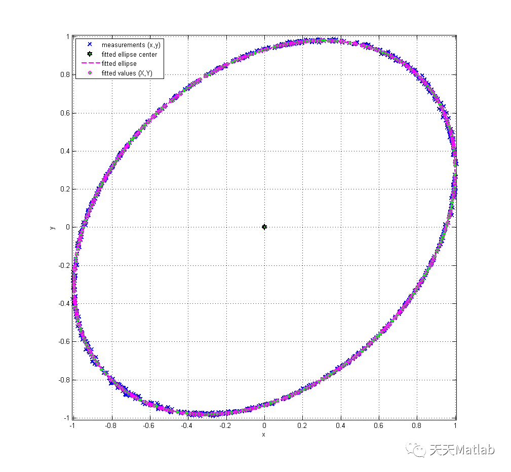
%% CORRELATED MEASUREMENTS
clear
%% GENERATE the correlated measurements: x and y
alpha0true = 0; % x-center (offset x)
beta0true = 0; % y-center (offset x)
alpha1true = 1; % x-amplitude
beta1true = 0.98; % y-amplitude
phi0true = pi/10; % phase offset
sigma = 0.005; % std of x and y independent errors
n = 1000; % number of measurements points
cycles = 1; % measurement interval, # cycles
phitrue = cycles*(2*pi)*sort(rand(n,1)); % true phases phi_i
% true values: X and Y
Xmean = @(t) alpha0true + alpha1true * cos(t);
Ymean = @(t) beta0true + beta1true * sin(t + phi0true);
rho = 0.9;
err = mvnrnd([0 0],sigma^2*[1 rho; rho 1],n);
% AR errors + correlated x and y
% rhoAR = -.99995;
% err = sigma*filter(1,[1 rhoAR],mvnrnd([0 0],[1 rho; rho 1],n));
x = Xmean(phitrue) + err(:,1);
y = Ymean(phitrue) + err(:,2);
%% Fit the ellipse based on measured data
options.alpha = 0.05;
options.correlation = rho; % Set the true correlation (assumed to be known)
options.displconst = 633.3/(4*pi);
options.displunit = 'nanometer [nm]';
result = ellipseFit4HC(x,y,options);
disp(result)
%% Display statistics of the fitted displacements (!! Table with n rows !!)
TABLE1 = result.TABLE_EllipsePars;
TABLE2 = result.TABLE_Displacements;
disp(TABLE2)
disp(['Displacement unit: ' result.Displacement_unit])
%% Plot the stat. uncertainty of displacement
displ_std = result.Displacement_std;
figure
plot(phitrue, displ_std)
xlabel('phi');
ylabel(['Statistical uncertainty of displacement, ',result.Displacement_unit]);
title(['Statistical Uncertainty: Min: ', ...
num2str(result.Displacement_std_min), ', Max: ', ...
num2str(result.Displacement_std_max) ]);
%% Plot the displacements with expanded uncertainties
displ_fit = result.Displacement_fit;
const = result.Displacement_const;
displ_true = const*phitrue;
displ_res = displ_fit - displ_true;
ix = (result.phi_fit-phitrue) < -1;
displ_res(ix) = displ_res(ix) + 2*pi*const;
figure
plot(displ_true, displ_res ,'o')
hold
plot(displ_true, 2*displ_std ,'r-')
plot(displ_true, -2*displ_std ,'r-')
grid
xlabel('True displacement');
ylabel('Displacement Residuals');
title('Expanded Uncertainty of Fitted Displacement');
%% Plot the X residuals with the expanded uncertainties
figure
plot(phitrue,result.x_res_fit,'.')
hold
plot(phitrue,2*result.x_res_std,'r-')
plot(phitrue,-2*result.x_res_std,'r-')
grid
xlabel('True phi');
ylabel('x residuals');
title('Expanded Uncertainty of Fitted X Residuals');
%% Plot the Y residuals with the expanded uncertainties
figure
plot(phitrue,result.y_res_fit,'.')
hold
plot(phitrue,2*result.y_res_std,'r-')
plot(phitrue,-2*result.y_res_std,'r-')
grid
xlabel('True phi');
ylabel('y residuals');
title('Expanded Uncertainty of Fitted Y Residuals');3 仿真结果
4 参考文献
[1]吴美容, and 王建国. "Matlab在离散点拟合椭圆及极值距离计算中的应用." 地矿测绘 32.4(2016):4.
博主简介:擅长智能优化算法、神经网络预测、信号处理、元胞自动机、图像处理、路径规划、无人机等多种领域的Matlab仿真,相关matlab代码问题可私信交流。
部分理论引用网络文献,若有侵权联系博主删除。