深度学习——02、深度学习入门 15-18

15Python环境搭建（推荐Anaconda方法）

​​软件万能安装起点​​

​​python官网​​

​​Anaconda官网​​

16Eclipse搭建python环境

​​软件万能安装起点​​

​​python官网​​

​​Eclipse官网​​

17动手完成简单神经网络

import numpy as np

def sigmoid (x,deriv=False):
    if(deriv==True):
        return x*(1-x)
    return 1/(1+np.exp(-x))

x=np.array([
    [0,0,1],
    [0,1,1],
    [1,0,1],
    [1,1,1],
    [0,0,1]
])
print(x.shape)
y=np.array([
    [0],
    [1],
    [1],
    [0],
    [0]
])
print(y.shape)

np.random.seed(1)

w0=2*np.random.random((3,4))-1
w1=2*np.random.random((4,1))-1

for j in range(100000):
    l0=x

    l1=sigmoid(np.dot(l0,w0))
    l2=sigmoid(np.dot(l1,w1))
    l2_error=y-l2
    if(j%10000)==0:
        print('Error'+str(np.mean(np.abs(l2_error))))
    l2_delta=l2_error*sigmoid(l2,deriv=True)
    l1_error=l2_delta.dot(w1.T)
    l1_delta=l1_error*sigmoid(l1,deriv=True)

    w1 += l1.T.dot(l2_delta)
    w0 += l0.T.dot(l1_delta)

代码分析

激活函数

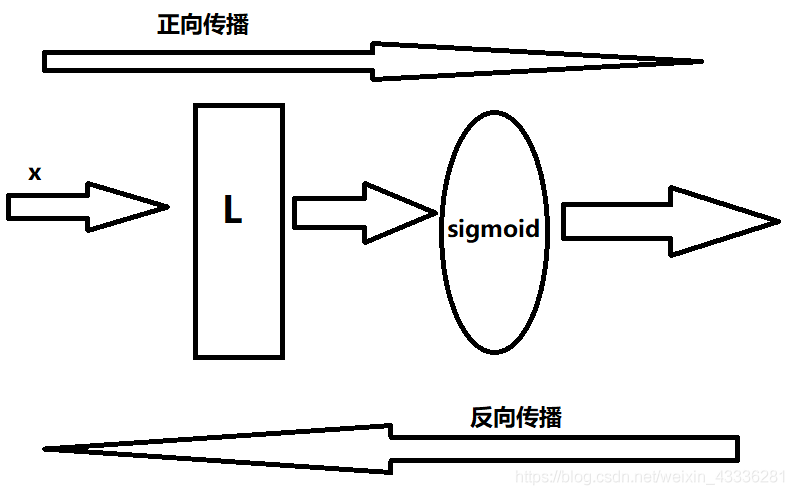
def sigmoid (x,deriv=False):
    '''
    激活函数
    :param x:
    :param deriv:标志位，当derive为假时，不计算导数，反之计算，控制传播方向。
    :return:
    '''
    if(deriv==True):
        # 求导
        return x*(1-x)
    return 1/(1+np.exp(-x))

激活函数参见：​​机器学习——01、机器学习的数学基础1 - 数学分析——Sigmoid/Logistic函数的引入​​

定义input和lable值

x=np.array([
    [0,0,1],
    [0,1,1],
    [1,0,1],
    [1,1,1],
    [0,0,1]
])
y=np.array([
    [0],
    [1],
    [1],
    [0],
    [0]
])

可以看一下x和y的维度：

print(x.shape)
print(y.shape)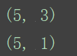

指定随机种子

np.random.seed(1)

保证数据一致，方便对比结果。

初始化权重值

#定义w0和w1在-1到1之间
w0=2*np.random.random((3,4))-1
#三行对应x的三个特征，四列对应L1层的四个神经元
w1=2*np.random.random((4,1))-1
#四行对应L1的四个神经元，一列对应输出0或1

定义三层神经网络

l0=x
    #L0层为输入层

    #进行梯度传播操作：
    l1=sigmoid(np.dot(l0,w0))
    #L0与W0进行矩阵运算得到L1
    l2=sigmoid(np.dot(l1,w1))
    #L1与W1进行矩阵运算得到L2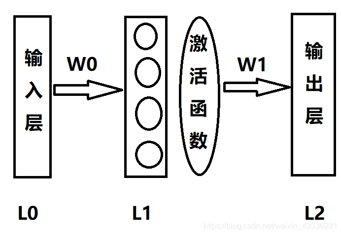

根据误差更新权重

l2_error=y-l2
    #预测值与真实值之间的差异
    if(j%10000)==0:
        print('Error'+str(np.mean(np.abs(l2_error))))
        #打印误差值
    l2_delta=l2_error*sigmoid(l2,deriv=True)
    #反向传播求导，差异值越大，需要更新的越大
    l1_error=l2_delta.dot(w1.T)
    #w1进行转置之后与l2_delta进行矩阵运算
    l1_delta=l1_error*sigmoid(l1,deriv=True)

    #更新w1和w2
    w1 += l1.T.dot(l2_delta)
    w0 += l0.T.dot(l1_delta)

18感受神经网络的强大

假设有如下数据要将其分类

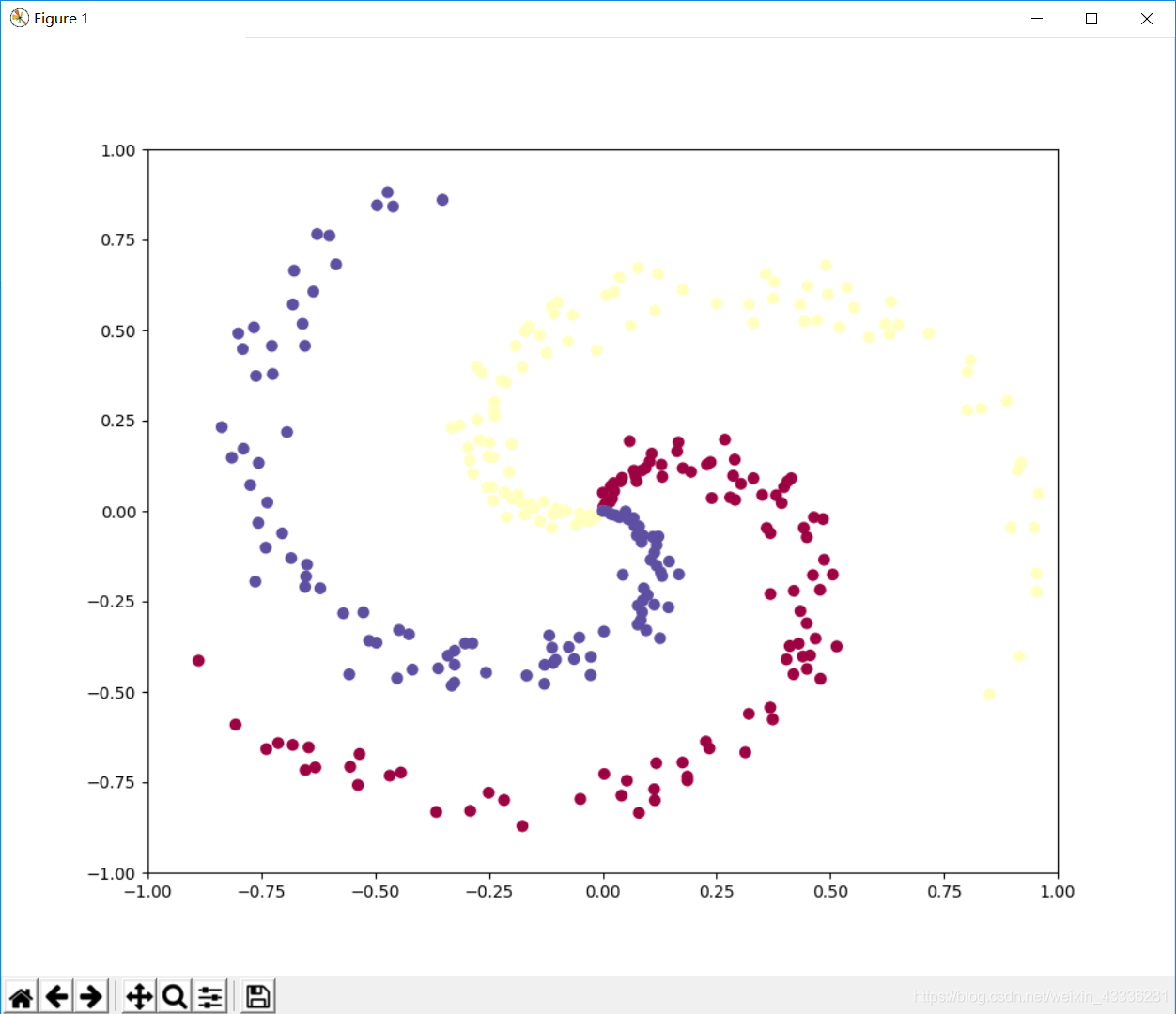
代码

import numpy as np
import matplotlib.pyplot as plt

#ubuntu 16.04 sudo pip instal matplotlib

plt.rcParams['figure.figsize'] = (10.0, 8.0) # set default size of plots
plt.rcParams['image.interpolation'] = 'nearest'
plt.rcParams['image.cmap'] = 'gray'

np.random.seed(0)
N = 100 # number of points per class
D = 2 # dimensionality
K = 3 # number of classes
X = np.zeros((N*K,D))
y = np.zeros(N*K, dtype='uint8')
for j in range(K):
  ix = range(N*j,N*(j+1))
  r = np.linspace(0.0,1,N) # radius
  t = np.linspace(j*4,(j+1)*4,N) + np.random.randn(N)*0.2 # theta
  X[ix] = np.c_[r*np.sin(t), r*np.cos(t)]
  y[ix] = j
fig = plt.figure()
plt.scatter(X[:, 0], X[:, 1], c=y, s=40, cmap=plt.cm.Spectral)
plt.xlim([-1,1])
plt.ylim([-1,1])
plt.show()

传统AI算法

#Train a Linear Classifier
import numpy as np
import matplotlib.pyplot as plt


np.random.seed(0)
N = 100 # number of points per class
D = 2 # dimensionality
K = 3 # number of classes
X = np.zeros((N*K,D))
y = np.zeros(N*K, dtype='uint8')
for j in range(K):
  ix = range(N*j,N*(j+1))
  r = np.linspace(0.0,1,N) # radius
  t = np.linspace(j*4,(j+1)*4,N) + np.random.randn(N)*0.2 # theta
  X[ix] = np.c_[r*np.sin(t), r*np.cos(t)]
  y[ix] = j



W = 0.01 * np.random.randn(D,K)
b = np.zeros((1,K))

# some hyperparameters
step_size = 1e-0
reg = 1e-3 # regularization strength

# gradient descent loop
num_examples = X.shape[0]
for i in range(1000):
  #print X.shape
  # evaluate class scores, [N x K]
  scores = np.dot(X, W) + b   #x:300*2 scores:300*3
  #print scores.shape 
  # compute the class probabilities
  exp_scores = np.exp(scores)
  probs = exp_scores / np.sum(exp_scores, axis=1, keepdims=True) # [N x K] probs:300*3
  print (probs.shape )
  # compute the loss: average cross-entropy loss and regularization
  corect_logprobs = -np.log(probs[range(num_examples),y]) #corect_logprobs:300*1
  print (corect_logprobs.shape)
  data_loss = np.sum(corect_logprobs)/num_examples
  reg_loss = 0.5*reg*np.sum(W*W)
  loss = data_loss + reg_loss
  if i % 100 == 0:
    print ("iteration %d: loss %f" % (i, loss))
  
  # compute the gradient on scores
  dscores = probs
  dscores[range(num_examples),y] -= 1
  dscores /= num_examples
  
  # backpropate the gradient to the parameters (W,b)
  dW = np.dot(X.T, dscores)
  db = np.sum(dscores, axis=0, keepdims=True)
  
  dW += reg*W # regularization gradient
  
  # perform a parameter update
  W += -step_size * dW
  b += -step_size * db
  scores = np.dot(X, W) + b
predicted_class = np.argmax(scores, axis=1)
print ('training accuracy: %.2f' % (np.mean(predicted_class == y)))

h = 0.02
x_min, x_max = X[:, 0].min() - 1, X[:, 0].max() + 1
y_min, y_max = X[:, 1].min() - 1, X[:, 1].max() + 1
xx, yy = np.meshgrid(np.arange(x_min, x_max, h),
                     np.arange(y_min, y_max, h))
Z = np.dot(np.c_[xx.ravel(), yy.ravel()], W) + b
Z = np.argmax(Z, axis=1)
Z = Z.reshape(xx.shape)
fig = plt.figure()
plt.contourf(xx, yy, Z, cmap=plt.cm.Spectral, alpha=0.8)
plt.scatter(X[:, 0], X[:, 1], c=y, s=40, cmap=plt.cm.Spectral)
plt.xlim(xx.min(), xx.max())
plt.ylim(yy.min(), yy.max())
plt.show()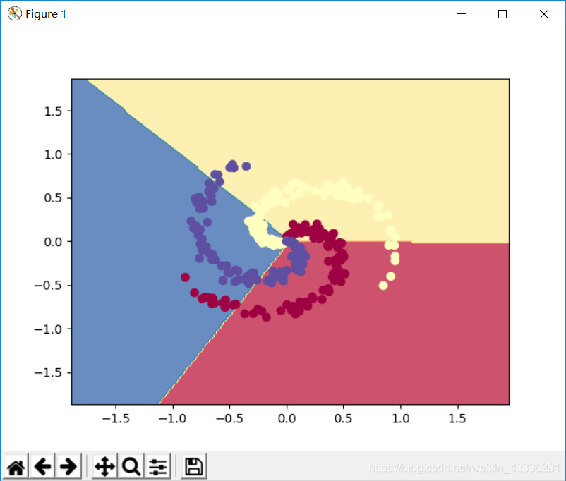

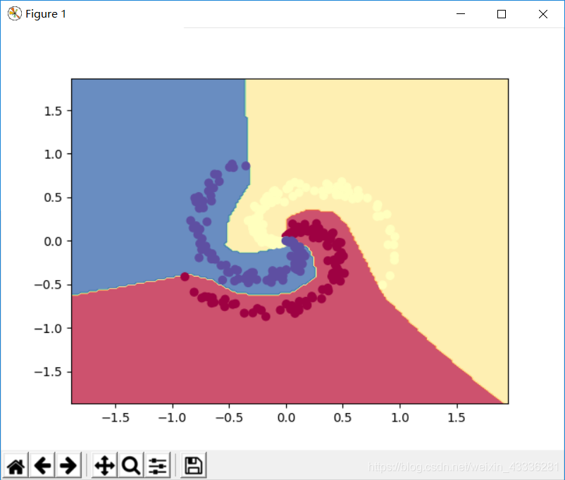
神经网络算法

import numpy as np
import matplotlib.pyplot as plt

np.random.seed(0)
N = 100 # number of points per class
D = 2 # dimensionality
K = 3 # number of classes
X = np.zeros((N*K,D))
y = np.zeros(N*K, dtype='uint8')
for j in range(K):
  ix = range(N*j,N*(j+1))
  r = np.linspace(0.0,1,N) # radius
  t = np.linspace(j*4,(j+1)*4,N) + np.random.randn(N)*0.2 # theta
  X[ix] = np.c_[r*np.sin(t), r*np.cos(t)]
  y[ix] = j
  
h = 100 # size of hidden layer
W = 0.01 * np.random.randn(D,h)# x:300*2  2*100
b = np.zeros((1,h))
W2 = 0.01 * np.random.randn(h,K)
b2 = np.zeros((1,K))

# some hyperparameters
step_size = 1e-0
reg = 1e-3 # regularization strength

# gradient descent loop
num_examples = X.shape[0]
for i in range(2000):
  
  # evaluate class scores, [N x K]
  hidden_layer = np.maximum(0, np.dot(X, W) + b) # note, ReLU activation hidden_layer:300*100
  #print hidden_layer.shape
  scores = np.dot(hidden_layer, W2) + b2  #scores:300*3
  #print scores.shape
  # compute the class probabilities
  exp_scores = np.exp(scores)
  probs = exp_scores / np.sum(exp_scores, axis=1, keepdims=True) # [N x K]
  #print probs.shape
  
  # compute the loss: average cross-entropy loss and regularization
  corect_logprobs = -np.log(probs[range(num_examples),y])
  data_loss = np.sum(corect_logprobs)/num_examples
  reg_loss = 0.5*reg*np.sum(W*W) + 0.5*reg*np.sum(W2*W2)
  loss = data_loss + reg_loss
  if i % 100 == 0:
    print ("iteration %d: loss %f" % (i, loss))
  
  # compute the gradient on scores
  dscores = probs
  dscores[range(num_examples),y] -= 1
  dscores /= num_examples
  
  # backpropate the gradient to the parameters
  # first backprop into parameters W2 and b2
  dW2 = np.dot(hidden_layer.T, dscores)
  db2 = np.sum(dscores, axis=0, keepdims=True)
  # next backprop into hidden layer
  dhidden = np.dot(dscores, W2.T)
  # backprop the ReLU non-linearity
  dhidden[hidden_layer <= 0] = 0
  # finally into W,b
  dW = np.dot(X.T, dhidden)
  db = np.sum(dhidden, axis=0, keepdims=True)
  
  # add regularization gradient contribution
  dW2 += reg * W2
  dW += reg * W
  
  # perform a parameter update
  W += -step_size * dW
  b += -step_size * db
  W2 += -step_size * dW2
  b2 += -step_size * db2
hidden_layer = np.maximum(0, np.dot(X, W) + b)
scores = np.dot(hidden_layer, W2) + b2
predicted_class = np.argmax(scores, axis=1)
print ('training accuracy: %.2f' % (np.mean(predicted_class == y)))


h = 0.02
x_min, x_max = X[:, 0].min() - 1, X[:, 0].max() + 1
y_min, y_max = X[:, 1].min() - 1, X[:, 1].max() + 1
xx, yy = np.meshgrid(np.arange(x_min, x_max, h),
                     np.arange(y_min, y_max, h))
Z = np.dot(np.maximum(0, np.dot(np.c_[xx.ravel(), yy.ravel()], W) + b), W2) + b2
Z = np.argmax(Z, axis=1)
Z = Z.reshape(xx.shape)
fig = plt.figure()
plt.contourf(xx, yy, Z, cmap=plt.cm.Spectral, alpha=0.8)
plt.scatter(X[:, 0], X[:, 1], c=y, s=40, cmap=plt.cm.Spectral)
plt.xlim(xx.min(), xx.max())
plt.ylim(yy.min(), yy.max())
plt.show()